Proceedings of the Sixth International Symposium on Combinatorial Search
Towards Rational Deployment of Multiple Heuristics in A* (Extended Abstract)
David Tolpin, Tal Beja
Solomon Eyal Shimony
CS Department
Ben-Gurion University
Israel
{tolpin,bejat,shimony}@cs.bgu.ac.il
Ariel Felner
Erez Karpas
ISE Department
Ben-Gurion University
Israel
felner@bgu.ac.il
IEM Department
Technion
Israel
karpase@gmail.com
Abstract
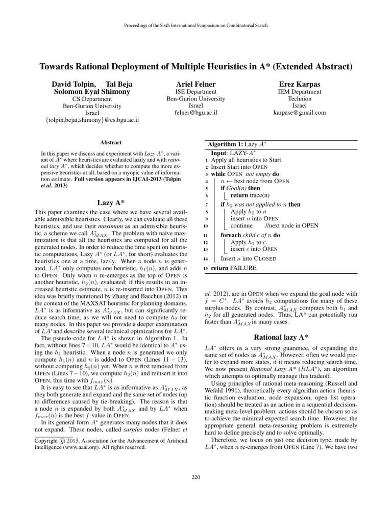
Algorithm 1: Lazy A∗
Input: LAZY-A∗
1 Apply all heuristics to Start
2 Insert Start into O PEN
3 while O PEN not empty do
4
n ← best node from O PEN
5
if Goal(n) then
6
return trace(n)
7
if h2 was not applied to n then
8
Apply h2 to n
9
insert n into O PEN
10
continue
//next node in OPEN
11
foreach child c of n do
12
Apply h1 to c.
13
insert c into O PEN
14
Insert n into C LOSED
15 return FAILURE
∗
In this paper we discuss and experiment with Lazy A , a variant of A∗ where heuristics are evaluated lazily and with rational lazy A∗ , which decides whether to compute the more expensive heuristics at all, based on a myopic value of information estimate. Full version appears in IJCAI-2013 (Tolpin
et al. 2013)
Lazy A*
This paper examines the case where we have several available admissible heuristics. Clearly, we can evaluate all these
heuristics, and use their maximum as an admissible heuristic, a scheme we call A∗M AX . The problem with naive maximization is that all the heuristics are computed for all the
generated nodes. In order to reduce the time spent on heuristic computations, Lazy A∗ (or LA∗ , for short) evaluates the
heuristics one at a time, lazily. When a node n is generated, LA∗ only computes one heuristic, h1 (n), and adds n
to O PEN. Only when n re-emerges as the top of O PEN is
another heuristic, h2 (n), evaluated; if this results in an increased heuristic estimate, n is re-inserted into O PEN. This
idea was briefly mentioned by Zhang and Bacchus (2012) in
the context of the MAXSAT heuristic for planning domains.
LA∗ is as informative as A∗M AX , but can significantly reduce search time, as we will not need to compute h2 for
many nodes. In this paper we provide a deeper examination
of LA∗ and describe several technical optmizations for LA∗ .
The pseudo-code for LA∗ is shown in Algorithm 1. In
fact, without lines 7 – 10, LA∗ would be identical to A∗ using the h1 heuristic. When a node n is generated we only
compute h1 (n) and n is added to O PEN (Lines 11 – 13),
without computing h2 (n) yet. When n is first removed from
O PEN (Lines 7 – 10), we compute h2 (n) and reinsert it into
O PEN, this time with fmax (n).
It is easy to see that LA∗ is as informative as A∗M AX , as
they both generate and expand and the same set of nodes (up
to differences caused by tie-breaking). The reason is that
a node n is expanded by both A∗M AX and by LA∗ when
fmax (n) is the best f -value in O PEN.
In its general form A∗ generates many nodes that it does
not expand. These nodes, called surplus nodes (Felner et
al. 2012), are in O PEN when we expand the goal node with
f = C ∗ . LA∗ avoids h2 computations for many of these
surplus nodes. By contrast, A∗M AX computes both h1 and
h2 for all generated nodes. Thus, LA* can potentially run
faster than A∗M AX in many cases.
Rational lazy A*
∗
LA offers us a very strong guarantee, of expanding the
same set of nodes as A∗M AX . However, often we would prefer to expand more states, if it means reducing search time.
We now present Rational Lazy A* (RLA∗ ), an algorithm
which attempts to optimally manage this tradeoff.
Using principles of rational meta-reasoning (Russell and
Wefald 1991), theoretically every algorithm action (heuristic function evaluation, node expansion, open list operation) should be treated as an action in a sequential decisionmaking meta-level problem: actions should be chosen so as
to achieve the minimal expected search time. However, the
appropriate general meta-reasoning problem is extremely
hard to define precisely and to solve optimally.
Therefore, we focus on just one decision type, made by
LA∗ , when n re-emerges from O PEN (Line 7). We have two
Copyright c 2013, Association for the Advancement of Artificial
Intelligence (www.aaai.org). All rights reserved.
220
Domain
miconic
sokoban-opt08
OVERALL
hLA
141
23
698
lmcut
140
25
697
Problems Solved
max
selmax
140
141
25
24
722
747
LA∗
141
26
747
RLA∗
141
27
750
hLA
0.13
3.94
1.18
lmcut
0.55
1.76
0.98
Planning Time (seconds)
max
selmax
LA∗
0.58
0.57
0.16
2.19
2.96
1.9
0.98
0.89
0.79
RLA∗
0.16
1.32
0.77
LA∗
0.87
0.04
0.27
GOOD
RLA∗
0.88
0.4
0.34
Table 1: Planning Domains — Number of Problems Solved, Total Planning Time, and Fraction of Good Nodes
options: (1) Evaluate the second heuristic h2 (n) and add the
node back to O PEN (Lines 7-10) like LA∗ , or (2) bypass the
computation of h2 (n) and expand n right way (Lines 11 13), thereby saving time by not computing h2 , at the risk of
additional expansions and evaluations of h1 .
The only addition of RLA∗ to LA∗ is the option to bypass
h2 computations (Lines 7-10). Suppose that we choose to
compute h2 — this results in one of the following outcomes:
1: n is still expanded, either now or eventually.
2: n is re-inserted into O PEN, and the goal is found without
ever expanding n.
Computing h2 is helpful only in outcome 2, where potential time savings are due to pruning a search subtree at the
expense of t2 (n). Since we do not know this in advance, we
calculate and use ph - the probability that h2 is helpful.
In order to choose rationally, we define a criterion based
on value of information (VOI) of evaluating h2 (n) in this
context. The following notations are used. b(n) is the
branching factor at node n, td is the to time compute h2
and re-insert n into O PEN thus delaying the expansion of n,
te is the time to remove n from O PENand ph the probability
that h2 is helpful.
As we wish to minimize the expected regret, we should
thus evaluate h2 just when (1 − b(n)ph )td < ph te and
bypass this computation otherwise. The complete derivation
appears in our full paper (Tolpin et al. 2013).
of the table shows the number of solved problems in each
domain. As the table demonstrates, RLA∗ solves the most
problems, and LA∗ solves the same number of problems as
selective max. Thus, both LA∗ and RLA∗ are state-of-theart in cost-optimal planning.
The middle part of the Table 1 shows the geometric mean
of planning time in each domain, over the commonly solved
problems (i.e., those that were solved by all 6 methods).
RLA∗ is the fastest overall, with LA∗ second. Of particular interest is the miconic domain. Here, hLA is very informative and thus the variant that only computed hLA is
the best choice (but a bad choice overall). Observe that both
LA∗ and RLA∗ saved 86% of hLM CU T computations, and
were very close to the best algorithm in this extreme case.
This demonstrates their robustness.
The rightmost part of Table 1 shows the average fraction of nodes for which LA∗ and RLA∗ did not evaluate
the more expensive heuristic, hLM CU T , over the problems
solved by both these methods. This is shown in the good
columns. We can see that in domains where there is a difference in this number between LA∗ and RLA∗ , RLA∗ usually performs better in terms of time. This indicates that
when RLA∗ decides to skip the computation of the expensive heuristic, it is usually the right decision.
Finally, Table 2 shows the total number of expanded and
generated states over all commonly solved problems. LA∗ is
indeed as informative as A∗M AX (the small difference is
caused by tie-breaking), while RLA∗ is a little less informed
and expands slightly more nodes. However, RLA∗ is much
more informative than its “intelligent” competitor - selective
max, as these are the only two algorithms in our set which
selectively omit some heuristic computations. RLA∗ generated almost half of the nodes compared to selective max,
suggesting that its decisions are better.
Experimental results
We experimented with LA* and RLA* on a number of domains but focus here on planning domains where we experimented with two state of the art heuristics: the admissible
landmarks heuristic hLA (used as h1 ) (Karpas and Domshlak 2009), and the landmark cut heuristic hLM CU T (Helmert
and Domshlak 2009) (used as h2 ). We experimented with all
planning domains without conditional effects and derived
predicates (which the heuristics we used do not support)
from previous IPCs.
Table 1 depicts the experimental results (for two of our
domains and the overall over all domains) for LA∗ and
RLA∗ to that of A∗ using each of the heuristics individually, as well as to their max-based combination, and their
combination using selective max (Selmax) (Domshlak et al.
2012). Selmax is an online learning scheme which chooses
one heuristic to compute at each state. The leftmost part
hLA
lmcut
A∗M AX
selmax
LA∗
RLA∗
Expanded
183,320,267
23,797,219
22,774,804
54,557,689
22,790,804
25,742,262
References
Carmel Domshlak, Erez Karpas, and Shaul Markovitch. Online
speedup learning for optimal planning. JAIR, 44:709–755, 2012.
A. Felner, M. Goldenberg, G. Sharon, R. Stern, T. Beja, N. R.
Sturtevant, J. Schaeffer, and Holte R. Partial-expansion A* with
selective node generation. In AAAI, pages 471–477, 2012.
Malte Helmert and Carmel Domshlak. Landmarks, critical paths
and abstractions: What’s the difference anyway? In ICAPS, pages
162–169, 2009.
Erez Karpas and Carmel Domshlak. Cost-optimal planning with
landmarks. In IJCAI, pages 1728–1733, 2009.
Stuart Russell and Eric Wefald. Principles of metereasoning. Artificial Intelligence, 49:361–395, 1991.
D. Tolpin, Tal Beja, S. E. Shimony, A. Felner, and E. Karpas. Towards rational deployment of multiple heuristics in A*. In IJCAI,
2013.
Lei Zhang and Fahiem Bacchus. Maxsat heuristics for cost optimal
planning. In AAAI, 2012.
Generated
1,184,443,684
114,315,382
108,132,460
193,980,693
108,201,244
110,935,698
Table 2: Total Number of Expanded and Generated States
221