Handling Overtraced Strokes in Hand-Drawn Sketches
Tevfik Metin Sezgin and Randall Davis
MIT Computer Science and Artificial Intelligence Laboratory
The Stata Center 235
Cambridge MA, 02139
{mtsezgin,davis}@csail.mit.edu
Abstract
Overtracing is the phenomenon in sketching of repeatedly drawing over previously drawn ink. It is a naturally appearing effect and is especially frequent in domains such as architectural drawings. Existing work
in sketch recognition focuses on sketches with nonovertraced strokes. In this paper, we describe a method
for generating geometric approximations of overtraced
strokes in terms of primitives including lines, non-selfintersecting polylines, ellipses and arcs. Our system
generates concise approximations for overtraced strokes
at an early stage in sketch processing, making it possible to use these concise descriptions in higher level processing and sketch interpretation systems.
Introduction
Freehand sketches are inherently informal and messy. Unlike clean, computer generated diagrams, manifestations
of abstract shapes are imprecise and highly variable in
sketches. One of the challenges in sketch recognition is the
ability to support this imprecision and high variability, of
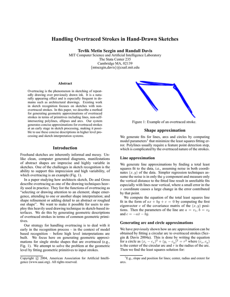
which overtracing is an example (Fig. 1).
In a paper studying how architects sketch, Do and Gross
describe overtracing as one of the drawing techniques heavily used in practice. They list the functions of overtracing as
“selecting or drawing attention to an element; shape emergence, attending to one or another shape interpretation; and
shape refinement or adding detail to an abstract or roughed
out shape”. We want to make it possible for users to employ this heavily used drawing technique in sketch-based interfaces. We do this by generating geometric descriptions
of overtraced strokes in terms of common geometric primitives.
Our strategy for handling overtracing is to deal with it
early in the recognition process – in the context of model
based recognition – before high level interpretations are
built. We focus here on generating geometric approximations for single stroke shapes that are overtraced (e.g.,
Fig. 1). We attempt to solve the problem at the geometric
level by fitting geometric primitives to input strokes.
c 2004, American Association for Artificial IntelliCopyright gence (www.aaai.org). All rights reserved.
Figure 1: Example of an overtraced stroke.
Shape approximation
We generate fits for lines, arcs and circles by computing
model parameters1 that minimize the least squares fitting error. Polylines usually require a feature point detection step,
which is complicated by the overtraced nature of the strokes.
Line approximation
We generate line approximations by finding a total least
squares fit to the data, i.e., assuming noise in both coordinates (x, y) of the data. Simpler regression techniques assume the noise is in only the y component and measure only
the vertical distance to the fitted line result in unreliable fits
especially with lines near vertical, where a small error in the
x coordinate causes a large change in the error contributed
by that point.
We compute the equation of the total least squares line
fit in the form of ax + by + c = 0 by computing the first
eigenvector v of the covariance matrix of the (x, y) positions. Then the parameters of the line are a = v1 , b = v2
and c = −ax̄ − bȳ.
Generating arc and circle approximations
We have previously shown how an arc approximation can be
obtained by fitting a circular arc to overtraced strokes (Sezgin & Davis 2004a). This is done by writing the equation
for a circle as (xi − cx )2 + (yi − cy )2 = r2 where (cx , cy )
is the center of the circular arc and r is the radius of the arc.
Then we find the least squares solution for:
1
E.g., slope and position for lines; center, radius and extent for
arcs.





2x1
2x2
.
.
2xn
2y1
2y2
.
.
2yn
1
1
.
.
1





"
cx
cy
r0
#



=

x1 2 + y1 2
x2 2 + y2 2
.
.
xn 2 + yn 2





100
80
2
Here r0 = r2 − cx 2 − cy 2 . Finally we calculate the starting angle and the extent for the arc. If the extent of the arc
computed by accumulating direction changes exceeds 2π,
we have a full circle instead of an arc.
60
40
Ellipse approximation
Among many methods for elliptical approximation of data
(Bookstein 1979; Fitzgibbon et al. 1999; Faber & Fisher
September 2001), we found the direct ellipse fitting method
proposed by (Fitzgibbon et al. 1999) to be the most appropriate, because it specifically attempts to fit an ellipse (as opposed to a generic conic section) to the data. It is also robust
enough for generating fits for point clouds. Their method
solves for the parameters of the generalized conic equation
ax2 + bxy + cy 2 + dx + ey + f = 0 subject to the constraint
4ac − b2 = 1 that results in an elliptical fit.
Alternatively, a simpler method that computes the parameters of an ellipse fit based on the rectangular bounding box
of the stroke can be used if the ellipses are known to be full.
Approximation of polylines
Existing work on polyline approximation uses speed and
curvature data as two sources of information to detect feature points,2 and relies on the data points to be sorted
along the path of the stroke (Sezgin et al. November 2001;
Calhoun et al. 2002; Bentsson & Eklundh 1992; Rattarangsi
& Chin 1992). In non-overtraced strokes, the time at which
points are sampled is implicitly assumed to give this ordering. Clearly, with overtraced strokes the timing information
cannot be used to order the points spatially, as points far
away temporally may end up close spatially.
Another challenge in dealing with overtraced polylines is
that due to the messy nature of sketching, ink in the overtraced parts of a stroke does not necessarily lie all on the
same line.
Feature point detection
We present a two step approach to feature point detection. In
the first step, we treat the input stroke as a collection of unordered points and apply a point cloud thinning approach
based on moving least squares method (Lee 2000) along
with the random sample consensus algorithm to move points
closer along a path perpendicular to the stroke. This gives
us a thinned version of the stroke. Next, we sort the points
along the stroke by an edge linking step that combines all the
points on a single path. Conventional feature point detection
methods can be applied from that point on. We begin with
the stroke thinning and point sorting processes.
2
Informally, feature points are the corners of a stroke, though
more generally they are defined as points in the stroke which separate curved or straight segments of a stroke.
20
0
160
180
200
220
240
260
280
300
Figure 2: The point cloud obtained by thinning the stroke
in Fig. 1. The ’+’ marks show the original locations of the
points in the stroke and the ’.’ marks show the locations after
thinning. The green dashed line shows the result of the edge
linking process.
Stroke thinning
Our approach to stroke thinning is based on the point cloud
thinning methods (Lee 2000). As seen in Fig.2, points in an
overtraced stroke fall in a band around the intended object.
The thinning process aims to bring these points closer to the
axis of the point cloud (i.e., to the shape that was possibly
intended by the user). In this respect, our method produces
shapes unlike the kinds of shapes produced by skeletonization and medial axis transforms.
Thinning is achieved by moving points in a direction perpendicular to the regression line obtained by fitting a line to
points in the local neighborhood of the point of interest. In
order to obtain reliable regression lines at the corners of a
shape, we employ a two step neighborhood selection technique.
Selecting a neighborhood
For each point pi to be moved during thinning, neighborhood selection determines the set of points to be used for
obtaining the local regression line towards which pi will be
moved. The usual approach in cloud thinning is to define
neighborhood as all points within a preset radius of pi . This
approach works well for smooth curves without sharp corners. For polylines or complex objects (i.e., combination
of lines and curves) our experiments show that this results
in unstable behavior at the corners, where the neighborhood
contains points from the edge containing pi and points from
the next edge. The points from the next edge act as distractors and the resulting linear regression line no longer becomes parallel to either of the edges forming the corner. This
is especially problematic for edges intersecting with acute
angles.
We solve this problem by employing a neighborhood selection scheme that is robust in the presence of large number
of outliers in the data. We use the random sample consen-
sus algorithm (Fischler & Bolles 1981) to select a subset of
points within a radius of pi that roughly lie on the same line.
We compute the linear regression line using these points.
Then pi is moved perpendicular to the regression line. After thinning, points less than a pixel apart are merged in a
greedy fashion to reduce the number of points.
Edge linking
After the point cloud is thinned, we connect individual
points to obtain a chain of points for the whole stroke. Although there are many solutions to this problem in the literature, we take a two step greedy approach. In the first step, we
connect each point to its closest neighbor. This gives us a list
of edges. We connect these edges starting with the ones that
have their end-points closest, obtaining longer point chains.
We continue this process until we are left with a single chain
linking all the points together.
The described thinning method also applies to complex
objects (i.e., combination of straight and curved segments).
Once the stroke is thinned and points are sorted, the corners (and the curved portions where applicable) of the resulting approximation can be detected using any curvature
based shape approximation method (Sezgin & Davis 2004b;
Sezgin et al. November 2001).
a. Original stroke.
140
120
100
80
60
Evaluation
We conducted a preliminary experiment running our algorithms on overtraced stroke data collected from 8 users using an Acer c110 Tablet PC. Although the data was collected
out of context, it served to be useful in detecting some of the
strengths and weaknesses of our approach.
We collected test data by asking each of the 8 users to
draw 5 overtraced examples of lines, circular arcs, circles,
ellipses, non-intersecting polylines and complex objects. In
each case, we visually compared the generated approximations to the shapes originally intended by the users. For the
stroke thinning method, we used a neighborhood radius of
20 pixels.
For primitive types where we could obtain direct least
squares fits (i.e., lines, arcs, circles and ellipses), in all cases
the computed approximations were in accordance with what
each user was asked to draw. This is an indication of the
robustness of direct fit methods.
The performance of our approach for polylines and complex shapes was also promising. For the majority of the
strokes, the thinning operation yielded the expected result
of aligning all the stroke points on a thin path. In a relatively
small number of cases (10% of the polylines and 12.5% of
the complex objects) the thinning operation failed to align
points. This caused the edge linking step to produce incorrect approximations. Fig.3 shows an example where this
occurs. After thinning Fig.3-a, we obtain the set of points
shown in Fig.3-b. As seen in Fig.3-b the thinned points on
the upper (negatively sloped) portion of the stroke don’t lie
on the same line.
This sort of behavior occurs when ink in a single segment of the stroke lies on two distinct clusters, and the radius
constant used for neighborhood computation fails to group
points in these clusters together.
40
220
240
260
280
300
320
340
b. Thinned and connected.
140
120
100
80
60
40
220
240
260
280
300
320
340
c. Original pen positions.
140
120
100
80
60
40
220
240
260
280
300
320
d. Original positions connected
with lines of uniform thickness.
Figure 3:
340
In Fig.3-c, the two distinct clusters are indicated using
blue and red dots. During the thinning process, for a number of points in these clusters, the neighborhood calculation
excludes points from the other cluster. As a result points on
one cluster get thinned using regression lines that are parallel but are a few pixels apart.
Related Work
Previous methods on stroke approximation assume that
points are sorted spatially along the stroke and use curvature
and pen speed information to detect feature points (Sezgin
et al. November 2001; Calhoun et al. 2002; Bentsson &
Eklundh 1992; Rattarangsi & Chin 1992). Cloud thinning
methods in the literature focus on smooth curves. Smooth
curves are generally easier to thin because they don’t need
the special neighborhood selection strategy similar to the
one we employ.
The stroke classification method described in (Shpitalni
& Lipson 2002) finds least squares solution of the generalized conic equation. For classification, it relies on classification heuristics such as signs and ratios of certain parameters in the conic equation. Furthermore, it assumes that each
stroke is a single entity (i.e., line, arc or a filleted corner).
Our approach doesn’t have this requirement and it is general
enough to be applicable to strokes that are combinations of
curved and straight segments. In addition, we obtain specific fits for each primitive class and suggest using the errors
of each type of fit as the goodness criteria as in (Sezgin et
al. November 2001) rather than performing the classification based on the relationship between the parameters that
solve a generic equation.
Future Work
As described in the evaluation section, in cases where an
individual segment of overtraced stroke forms parallel clusters within itself, the thinning operation fails to group the
points on a single line. This problem can be fixed by recursively applying the thinning operation with a stopping criteria based on the stability of points which says if a point
cloud becomes stable (i.e., if the points don’t get moved significantly by subsequent thinning operations), this may be
used as an indication that we converged on a solution. The
challenge would be in defining what constitutes as a “significant” change in point positions.
Another direction would be to investigate if factors, other
than the pen positions, which affect the way a stroke is rendered to the user can be used during the thinning process.
Such factors are especially important, because among other
things, they potentially determine how much overtracing a
user does (e.g., until the overtraced region is mostly covered with ink). Pen pressure is an example of information
other than pen positions that affects rendering. For example,
our data collection program renders strokes thicker at points
with high pen pressure. This is part of the reason why the
clusters in the negatively sloped part of the stroke in Fig.3a are more apparent in Fig.3-c and d, where we only show
the sampled points and connect them with uniform-thickness
lines; and less apparent in Fig.3-a. In Fig.3-a, lines connect-
ing the few points between the two clusters is thick enough
to close the gap between the two clusters visually. Pressure information can either be used to dynamically adjust
neighborhood parameters or it can be used to weigh points
with higher pen pressure more heavily using a weighted least
squares linear regression method.
The methods we presented worked well for the data collected in an isolated fashion (i.e., outside the context of a
specific sketching task or domain). On one hand this is justifiable because our aim has been to do low level processing
in a domain and task independent fashion. On the other hand
it is conceivable that overtracing behaviors differ across domains. Studying the extent to which this is true and determining what kinds of techniques can be adapted in these situations remains as an interesting area to explore.
References
Bentsson, A., and Eklundh, J. 1992. Shape representation
by multiscale contour approximation. IEEE PAMI 13, p.
85–93, 1992.
Bookstein, F. L. 1979. Fitting conic sections to scattered
data. Comput. Graphics Image Processing, vol. 9, pp. 5671.
Calhoun, C.; Stahovich, T. F.; Kurtoglu, T.; and Kara,
L. B. 2002. Recognizing multi-stroke symbols. In AAAI
2002Spring Symposium Series, Sketch Understanding.
Faber, P., and Fisher, R. B. September 2001. A buyer’s
guide to euclidean elliptical cylindrical and conical surface
fitting. Proc. British Machine Vision Conference BMVC01,
Manchester, pp 521-530.
Fischler, M. A., and Bolles, R. C. 1981. Random sample
consensus: A paradigm for model fitting with applications
to image analysis and automated cartography. Comm. of
the ACM, Vol 24, pp 381-395.
Fitzgibbon, A.; Pilu, M.; and Fisher, R. B. 1999. Direct
least squares fitting of ellipses. IEEE Pattern Analysis and
Machine Intelligence Vol 21, No 5.
Lee, I.-K. 2000. Curve reconstruction from unorganized
points. Computer aided geometric design 17 pp. 161-177.
Rattarangsi, A., and Chin, R. T. 1992. Scale-based detection of corners of planar curves. IEEE Transactionsos
Pattern Analysis and Machine Intelligence 14(4):430–339.
Sezgin, T. M., and Davis, R. 2004a. Early sketch processing with application in hmm based sketch recognition.
MIT Computer Science and Artificial Intelligence Laboratory Memo AIM-2004-016.
Sezgin, T. M., and Davis, R. 2004b. Scale-space based
feature point detection for digital ink. In AAAI 2004 Fall
Symposium Series, Sketch Understanding.
Sezgin, T. M.; Stahovich, T.; and Davis, R. November
2001. Sketch based interfaces: Early processing for sketch
understanding. Proceedings of PUI-2001.
Shpitalni, M., and Lipson, H. 2002. Classification of sketch
strokes and corner detection using conic sections and adaptive clustering. AAAI Spring Symposium: Sketch Understanding, March 25-27, Stanford CA.