The NFL Coaching Network: Analysis of the Social Network Among Professional
Football Coaches
Andrew Fast and David Jensen
Department of Computer Science
University of Massachusetts
Amherst, MA 01003
afast@cs.umass.edu, jensen@cs.umass.edu
Abstract
The interactions of professional football coaches and teams
in the National Football League (NFL) form a complex social
network. This network provides a great opportunity to analyze the influence that coaching mentors have on their protegés. In this paper, we use this social network to identify
notable coaches and characterize championship coaches. We
also utilize the coaching network to learn a model of which
teams will make the playoffs in a given year. Developing
comprehensive models of complex adaptive networks, such
as the network of NFL coaches, poses a difficult challenge
for researchers. From our analysis of the NFL, we identify
three types of dependencies that any model of complex network data must be able to represent.
Introduction
At the end of every National Football League (NFL) season,
underperforming teams seek to improve their prospects for
the upcoming season by making changes in their coaching
staff. Teams generally consider many characteristics of a
coaching candidate including personality, the type of “system” a coach runs, how a coach relates to players and many
others. Ultimately, teams seek the coach with the combination of skills that will help the team win the most games in
the future.
That combination, however, is difficult to determine and
teams often resort to other methods of choosing coaches.
The primary alternative is examining a coach’s coaching
“ancestry”; examining who the candidate has worked
with in the past and whether those mentors are successful
coaches. Considering this social aspect of coaching gives
rise to coaching trees. Like family trees, coaching trees
record the coaching ancestors and descendants for each
coach. Coaching trees are often cited by fans and the media
alike in the context of hiring a new coach or discussing the
accomplishments of a well regarded coach. Rather than
considering coaching trees individually, the work presented
in this paper examines the network of overlapping coaching
trees to identify characteristics of successful coaches and
the NFL as a whole.
c 2006, American Association for Artificial IntelliCopyright gence (www.aaai.org). All rights reserved.
Understanding this network has important implications
not only for observers of the game but also for those
seeking to improve the rate of minority hiring in the NFL.
The league has encouraged the consideration of minority
coaching candidates through the implementation of the
so-called Rooney rule which requires teams to interview at
least one minority candidate for any head coach opening.
Despite this rule and recent minority hirings, minority
coaches continue to be underrepresented. Michael Smith of
ESPN.com writes that the minority hiring problem is not
an issue of finding talented minority coaches but rather an
issue of networking as teams tend to hire familiar coaches
instead of unknown candidates. (Smith 2006)
In this paper we analyze the network of NFL coaches and
teams to learn statistical models of successful coaches with
the goal of understanding how the coaching network influences the hiring and success of coaching candidates. In the
following sections, we present a number of facts and models that begin to identify the significant interactions in the
NFL and suggest important facts for teams to consider when
making coaching decisions. Finally, we propose an initial
joint model of the variables that characterize the coaches and
teams in the NFL and discuss the necessary components of
models of complex adaptive networks, such as the network
of NFL coaches.
Data Description
The data consist of the network of NFL coaches and teams
dating back to the inception of the NFL in 1920 through the
conclusion of the 2005 season, the most recent NFL season.
This data are limited to the coaches who have been affiliated
with at least one of the 32 existing franchises. In the early
days of the league there were many franchises that only existed for a few seasons. While interesting from a historical
perspective, we do not consider the coaching staffs of those
teams. For the purposes of our analysis, we considered franchises that have changed cities over the years to be a single
entity. For example, the Tennessee Titans used to play in
Houston and were called the Oilers but are considered to be
the same franchise. For each franchise, we have a record of
the head coaches, assistant coaches, and win-loss-tie record
for every season that the franchise has fielded a team. In
addition, the data incorporates playoff information for every
season from 1920 through 2005. From 1970 to the present,
name
college
●
name
name
name
years_under
●
●
1940
1960
(a)
Overview of Coaching Networks
Figure 3 shows the network of mentor relationships among
championship coaches in the NFL. This figure contains all
coaches who have won a league or conference championship
game and any non-championship coach who has worked
with at least two championship coaches. Using an off-theshelf hierarchical graph layout 2 , Paul Brown was placed
at the top of the graph. This is not a surprise given that
Paul Brown was the founding coach of two different NFL
franchises and is responsible for introducing football as it is
known today. In an interview with the Boston Globe, Bill
Belichick, head coach of the New England Patriots and no
stranger to winning, called Paul Brown “the greatest innovator as a coach the game has ever had...Every single thing he
did was geared to maximize a team’s performance in terms
of winning” (Ryan 2005). This innovation is plainly evident
as Paul Brown’s influence is traced through his coaching descendants (including Belichick himself) touching almost every corner of the graph. One innovation that Paul Brown is
known for is the West Coast Offense. This offense is based
on movement and precisely timed plays and has changed the
way the game is played. Bill Walsh, one of Paul Brown’s
disciples, helped to perfect the West Coast offense and led
the San Francisco 49ers to three Super Bowl titles in the
1980’s and 1990’s (in addition to two more Super Bowls
after Walsh’s retirement). Bill Walsh’s coaching tree can be
found at the lower left of Figure 3. Note the four Super Bowl
winners that trace their coaching lineage to Bill Walsh.
As the NFL has grown and become more specialized,
the size of the coaching staff has also increased. The typ1
2
www.footballreasearch.com
www.graphviz.org
●
●
●
●●
●
●
●
●
●
●
●● ●
●
● ●● ●
●
●
●
●
●
●
●
●
● ●
● ●
● ● ● ● ●●
●
● ●
● ●
● ●
●
●
●●
●
●
●●
●
●●
●●
●
● ●
●
●
●
●●● ●
●
● ● ●●
●● ● ● ●
● ●●
●●● ●
●
●
●
●●
●●
●
●●
●● ●●
●●
●
●
●● ● ●
●●
●● ●
● ●
●
●
●● ●
●
●
●
● ● ● ●● ●
●●
●
● ●
●
●●
●●
● ●
●●
●●● ●●●●
● ● ●●
●
●
●●
●● ●●●
●
●
●●
●
●●
● ● ●
● ●●
●●
●●
● ●● ● ●
●●
●● ● ● ●●●● ●
●
●
●
●
●
First Year In League
the data also contain the number of points scored and the
number points allowed by a team. The coaching staffs of
each team through the 2000 season were provided by the
Professional Football Research Association 1 . The win-loss
and playoff records of each team were obtained from profootball-reference.com. A graphical representation of the
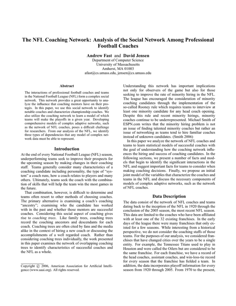
data schema can be viewed in Figure 1.
●
●●
●
1980
2000
10
●
8
●
●
●
●● ● ●●● ●● ●● ●●●
1940
●
●
●
●
●●●
●
●
●
●● ● ●
●
●
● ●●
●
●
● ● ●●●●● ●● ●●● ●●● ●
●●●● ● ●● ● ●● ● ● ●●●●● ●●
●●● ●●● ●●
●● ●● ● ●●●●
●
●
●
● ●● ●
●
●
1920
●
● ●●
● ●
●
●
●●●
●
●
●● ● ●
●
●
●
6
●
● ●
●
●
● ●
●
●●
●
●
●
●
●●
●
●
●
4
●
●
●
●
●
Number of Head Coaches
●
●
●
●
● ●
2
●
●
1920
Figure 1: The entities, relations and attributes of the NFL
coaching network from 1920 to the present
●
●
●
●
10
(32)
work_under
(5005)
●
●
●
●
●
●
●●
0
Franchise
(2)
Division
(8)
●
0
owned_by
12
60
(1840)
50
(15676)
●
●
●
40
Coach
30
coach_of
●
Conference
●
●
●
(1617)
plays_in
Head Coaches Produced
14
70
Growth of Coaching Staffs
Team
Number of Proteges
plays_in
position
years w/ team
year
20
name
year
wins
losses
ties
points-for
points-against
made-playofffs
won-super-bowl
●●
●
●● ●●●●●
●●● ● ●● ● ●●●●●●●●●●●● ●● ●●●
●●● ●● ●●●● ●●● ●
●●
●●
1960
●
● ● ●● ● ● ●● ●
● ● ●● ●● ●● ●●
1980
●
● ●●
2000
First Year In League
(b)
Figure 2: (a) This plot demonstrates the growth of coaching
staffs in NFL over time (b) Despite the growth in coaching
staff size shown in (a), the number of coaches produced by
the most prolific coaches remains consistent over time.
ical staff now includes coaches for strength and conditioning, defensive quality control, and others in addition to the
more traditional offensive coordinators, defensive coordinators and position coaches (Battista 2006; Liu & Marini
2004). This has led to a large increase in the number of assistant coaches that a head coach mentors over the course of
his career (See Figure 2(a)). While there has been marked
growth in the number of coaches mentored over time, the
number of coaches produced by the most prolific coaches
remains consistent over time. (Figure 2(b)). Table 1 lists the
coaches who have produced five or more head coaches and
have also won three or more championships. These coaches
are responsible for more than half of all Super Bowl victories (24/40).
Understanding the Network of NFL Coaches
As mentioned above, the network of coaches plays prominently into hiring decisions in the NFL. Unfortunately, it is
difficult to know in advance if hiring a particular coach is a
good idea. Some coaches vastly exceed expectations while
others never live up to their potential. We seek to develop
models of the network among NFL coaches to better infer
characteristics of coaches based on their interactions with
other coaches as well as their performance with previous
coaching positions. The NFL coaching network is an example of a broader class of complex adaptive networks that
are often of interest to researchers. In addition to inferring
characteristics of coaches, we seek to learn how the interactions among a coaching staff influence the performance of
their team in a given year. In this paper, we highlight interactions among coaches and teams that begin to describe the
types of dependencies present in these data. First, we examine the relationships between coaches and their mentors and
characterize the influence that championship coaches have
on their protegés. Second, we utilize the network of coaches
to make predictions about the playoff success of teams.
P. Brown
B. Shaw
B. Collier
J. Williams
E. Khayat
R. Parker
N. Skorich
S. Owen
H. Gilmer
R. Flaherty
J. Howell
T. Landry
E. Biles
T. Prothro
W. Ewbank
S. Gillman
C. Knox
B. Peterson
D. Vermeil
H. Stram
J. Johnson
N. Turner
R. Kotite
D. Reeves
R. Brooks
M. Ditka
B. Grant
R. Rhodes
J. Gruden
B. Callahan
H. Taylor
M. Levy
M. Campbell
W. Phillips
J. Rauch
D. Green
M. White
B. Cowher
C. Studley
A. Shell
B. Parcells
M. Mularkey
R. Erhardt
B. Billick
R. Handley
J. Fassel
J. Fox
J. Gibbs
T. Flores
R. Perkins
H. Svare
D. Shula
L. Saban
B. Belichick
E. Lambeau
G. Neale
B. Snyder
J. Stydahar
B. McPeak
L. Rymkus
W. Lemm
F. Gregg
M. Speedie
J. Robinson
A. Walsh
C. Shaughnessy
C. Noll
R. Waller
H. Devore
M. Holovak
W. Kiesling
M. McCormack
J. McKay
J. Madden
S. Wyche
G. Wilson
P. Bengtson
D. McCafferty
V. Tobin
G. Seifert
A. Reid
G. Allen
B. Ryan
B. Walsh
M. Shanahan
V. Lombardi
A. Davis
M. Martz
M. Holmgren
G. Halas
R. Forzano
D. Modzelewski
R. Malavasi
J. Fisher
J. Faulkner
J. Dooley
L. Steckel
J. Pardee
B. Ross
H. Bullough
R. Berry
L. Johnsos
H. Anderson
Figure 3: The network among championship coaches in the NFL. The dark grey (red) nodes indicate coaches who have won
a Super Bowl. Light grey (green) indicates a league championship victory. White nodes indicate coaches with no championships or Super Bowls. The graph includes all championship coaches and additional coaches who are connected to 2 or more
championship coaches. Links indicate the work-under relation and point from the head coach to his assistants.
Name
George Halas
Weeb Ewbank
Vince Lombardi
Tom Landry
Chuck Noll
Don Shula
Bill Walsh
Hank Stram
Bud Grant
Marv Levy
Dan Reeves
Bill Belichick
Joe Gibbs
Bill Parcells
Mike Holmgren
First Year
1920
1949
1954
1954
1960
1960
1960
1960
1967
1969
1970
1976
1978
1979
1986
Num. Years
Head Coach
40
20
10
29
23
33
10
17
18
17
23
11
14
18
14
Playoffs
Champs
9
4
6
18
12
19
7
5
12
8
9
5
9
9
10
5
3
5
5
4
6
3
3
4
4
4
3
4
3
3
Super
Bowls
0
1
2
2
4
2
3
1
0
0
0
3
3
2
1
Proteges
Head Coaches
Produced
11
11
7
9
6
9
9
7
7
9
10
6
6
9
7
22
23
17
27
35
39
23
22
19
36
66
45
41
47
41
Betweenness
19078
21241
1515
21159
32590
37071
33558
18935
6936
20803
60265
51311
21533
29559
42420
Table 1: Coaches who produced 5 or more head coaches and won 3 or more championships. These 15 coaches account for
more than half of all Super Bowl victories (24/40).
Identifying Championship Coaches
0.25
Mentors of Championship Coaches
Density
0.05
0.10
0.15
0.20
Champ. Coaches
Non−Champ. Coaches
0.00
As in most professions, the performance of an NFL head
coach depends on the skills developed while training. We
examined a number of characteristics of the coaches who
mentor assistant coaches trying to understand how a coach
becomes a championship coach. For our purposes we
considered a championship coach to be someone who has
coached in a Super Bowl or won a league championship
prior to the creation of the Super Bowl in 1967. Sometimes
it is said that coaches are “paying their dues” working as
an assistant coach for a number of years with a few different teams before becoming a head coach. It is reasonable
to expect that a coach who has worked under a number of
mentors would have gathered a broad range of skills and experience making him a prime candidate for a head coaching
position. We found this not to be the case in the NFL through
the 2005 season. Championship coaches work with significantly fewer (p ≤ 0.001) mentors than non-championship
coaches. (See Figure 4). Instead of “paying dues” , the most
talented assistant coaches tend to stay with a single mentor
until they are promoted into a head coaching position.
Given that successful coaches only work for a small number of mentors, if we can characterize those mentors then
it would be possible to identify prospective championship
coaches. As is evident in Figure 5(a), there are two types
of championship coaches: those who produce many future
head coaches (≥ 5) and those who do not. Out of 61 championship coaches recorded in the data, 30 produced five or
more future head coaches and 31 produced fewer than five
future head coaches. Intuitively, it is expected that coaches
who mentor many future head coaches are also likely to produce many future championship coaches. Figure 5(b) confirms that intuition for the NFL. Using a linear regression
model, we can estimate the dependency between the number of future championship coaches a coach will produce
and the number of head coaches produced. The slope of the
regression line is significant (p ≤ 0.001).
0
5
10
15
Number of Mentors
Figure 4: Distribution of the number of mentors of championship and non-championship coaches. Head coaches who
win championships have significantly fewer mentors than
non-championship coaches. (p ≤ 0.001)
Because coaches who produce many head coaches also
produce many championship coaches, we learned a conditional probability model to characterize those coaches who
have produced five or more head coaches. This model
is shown in Figure 6. Our model was learned using the
relational probability tree (RPT) algorithm (Neville et al.
2003). Designed with heterogeneous data in mind, the RPT
searches over possible aggregations and thresholds of attributes appearing in the data. For example, over his career
a coach will work for a number of teams. Possible aggregations include but are not limited to the number (or degree) of
teams a coach has worked for, the average number of wins
of a coach’s teams, or the maximum number of wins scored
by any team a coach has worked for. In the NFL data, the
feature ranked most highly by our model is the degree of
Degree >= 10.0
(Team)
Future Champions
5
Prolific Coaches
Champ. Coaches
Non−Champ. Coaches
●
Y
3
●
Count >= 5
2
(PastTeam.wins <= 4)
0
−2
0
2
4
6
8
Head Coaches Produced
(a)
10
12
N
●
●
●
●
●
●
●
●
●
●
●
●
●
●
P(+) = 0.10
(19)
●
Y
0.00
Density
●
1
0.05
0.10
0.15
Future Champs Produced
4
0.20
Champions
Non−Champions
●
0
●
●
2
●
●
4
●
●
●
6
8
10
12
N
14
Head Coaches Produced
(b)
Figure 5: (a) This plot compares the number of head
coaches produced by championship coaches to the number
of head coaches produced by non-championship coaches.
(b) Coaches that produce many head coaches also produce
many future championship coaches. The slope of the regression line is significant (p ≤ 0.001). See Table 1 for championship coaches who produce many future head coaches.
P(+) = 0.2
(3)
P(+) = 0.89
(26)
Figure 6: This is a learned relational probability tree (RPT)
which characterizes coaches who have produced five or
more head coaches using the attributes of a coach, the attributes of the teams he has coached, and the attributes of his
mentors. Features are computed by aggregating attributes
on particular related objects and are identified by EntityName.attribute. Probabilities are Laplace corrected values.
Identifying Playoff Teams
teams that a coach has worked for, with a threshold of ten
seasons. As expected, successful coaches spend more years
as a head coach than unsuccessful coaches. It is rare for
a team to fire a coach who produces winning teams, and
championship coaches who happen to be unemployed typically do not stay unemployed for long. It is rare for a coach
produce five or more championship coaches and have won
a championship after having been a head coach for ten or
fewer years. If they have worked for at least ten years as a
head coach, then the next best feature selected by our model
is the count of teams that have won fewer than four games
in a season. A NFL season is 16 games long, a team that
wins four or fewer games is typically at the bottom of its
conference. If a coach has had five or more teams that won
four or fewer games, then that coach is not likely to be successful over the long term and consequently won’t produce
many future head coaches. Note that very few coaches in
the NFL data fall into this category. As expected, the majority of championship coaches tend to coach for many years
and coach winning teams. This model performs with accuracy of 0.804 and area under the ROC curve (AUC) of
0.811. As shown in Figure 6, a feature consists of the aggregator and value used to compute the feature score and
the entity, attribute and threshold that the score is computed
over. We use EntityName.attribute to distinguish between
similarly named attributes on different object types.
Unfortunately, this model does not provide much help in
suggesting methods for identifying good coaching mentors.
The input to the model included many attributes of coaches
including wins and playoff performance. Since those feature were not chosen by the model, it implies that different coaches have different recipes for winning, and winning
coaches continue to have jobs in the NFL.
Each year NFL teams construct their coaching staff in order
to maximize their chances of making it to the playoffs and
winning the Super Bowl. Using the social network among
coaches, we can empirically determine the effect a coaching staff has on the playoff success of teams. Obviously,
the performance of teams in any given season also depends
greatly on the players involved. However, we demonstrate
that coaching histories have a significant effect on a team’s
probability of making the playoffs. (See Figure 7).
We learned a conditional model predicting which teams
will make the playoffs given the coaching histories of the
coaching staff for that year. Our model considered the attributes of the head coaches, assistant coaches, each of the
past teams that those coaches have worked for and any mentor coaches they have worked under. As described in the
previous section, we used the relational probability tree algorithm to learn this model. The model, shown in Figure
8, identifies a number of factors which determine a team’s
playoff success. This model also introduces some new notation. HeadCoach->PastTeam indicates an aggregation over
PastTeams coached by the head coach.
The feature with the highest score in our model is
HeadCoach.year with team <= 1. Not surprisingly, teams
coaches by first-year coaches tend not to make the playoffs. If a coach has been with a team for more than one
season, then the features selected by our model are aggregations of past playoff performance and coaching experience.
Our model shows that the experience of the assistant coaches
also contributes to the success of team. If a team has assistant coaches who have made the playoffs at least 34% of
the time, then the probability of that team making the playoffs is increased. It is also interesting that mentor coaches
have an effect on playoff success. If a team has a first-year
Count >= 1
HeadCoach.
year_with_team <= 1.0
Predicting Playoff Success
N
1.0
Y
Proportion >= 1.0
Proportion >= 0.667
HeadCoach->PastTeam
.made_playoffs = 0
HeadCoach.
year_with_team <= 1.0
0.8
Proportion >= 0.34
HeadCoach->PastTeam
.year_with_team <= 1.0
AsstCoach->PastTeam
.made_playoffs = 1
N
0.6
0.4
0.2
Precision at Playoff Level
Count >= 5.0
HeadCoach->Mentor.
champ_coach = 0.0
P(+) = 0.04
(30)
0.0
1970
1975
1980
1985
1990
1995
2000
2005
N
Proportion >= 0.833
Y
Coaching History
Previous Year
Random
Y
N
Y
P(+) = 0.21
(126)
P(+) = 0.02
(41)
Y
P(+) = 0.75
(2)
N
P(+) = 0.10
(48)
Y
P(+) = 0.55
(261)
N
P(+) = 0.39
(308)
Figure 8: This is a learned relational probability tree model
which models the probability of a team making the playoffs
based on the coaching staff, previous teams that the coaching staff has coached, and mentor coaches. Probabilities reported are Laplace corrected values.
Season
Figure 7: Success of our learned model predicting playoffs
appearances by teams between 1970 and 2005. The precision at playoff level is the number of teams correctly predicted to be in the playoffs divided by the number of playoff
teams for each year.
coach who has a high proportion of mentors who have won
championships then the probability of that team making the
playoffs increased. While success in the first year is limited,
teams who hire accomplished coaching staffs should expect
to be successful within a few years.
We evaluated this model using precision at playoff level.
In each season there are a limited number of teams that
make the playoffs from each conference (e.g., in recent
seasons, six teams from each conference make the playoffs).
The precision of the model is the number of teams correctly
predicted to be in the playoffs divided by the number of
playoff teams for each year. Like a sportswriter making
pre-season playoff picks, precision at playoff level evaluates
how many of our “pre-season picks” went on to make
the playoffs. We ranked the teams from each conference
according to our model and selected our playoffs picks
from the top of each ranking. If multiple teams were tied
for the final playoff spot in a conference, we computed the
expected precision of filling that spot by choosing randomly
among the tied teams. On historical data from 1970 through
2005, our model achieves 0.63 mean precision at playoff
level. We compare our model against two baselines: a
simple model which simply predicts the same results as
the team in the previous year (0.57 mean precision) and an
analytical computation which computes the precision when
picking playoffs teams at random without replacement (0.37
mean precision). When comparing the means with a t-test,
our learned model performs significantly better (p ≤ 0.03)
than just predicting last year’s results.
One of the popular credos of NFL fans is that on “any
given Sunday” any team can beat any other team. Despite
this credo, it is often the case that playoff teams remain constant from year to year. Both our model of playoff success
and the simple model of using the previous year rely on this
fact to make successful predictions. Based on the results of
our model it appears that playoff consistency is in decline.
There are three distinct eras of NFL history that appear in
Figure 7. The first era occurs between 1970 and 1982. The
modern NFL was created in 1970 by the merger of NFL
with the American Football League (AFL), an upstart conference founded in 1960. In this era, there was strong consistency among the playoff teams from year to year which
allows the previous year model as well as our coaching history model. In 1982, there was a strike by the players which
resulted in a short season and an expanded playoff field that
increased the chance that a team would make the playoffs.
The NFL allowed free agency in 1992 and implemented a
cap on team payroll (i.e., a salary cap) in 1994. Based on
the performance of the RPT model, coaching histories have
the most effect on playoff performance in years with significant change in the NFL. In 1982 and 1990 the playoff field
was expanded, 1992 marks the start of free agency, and 1994
marks the start of the salary cap. In each of those years, our
model based on coaching histories out performed the previous year model. After the salary cap took effect in 1994,
the predictive capability of both our model and the previous
year model begins to decrease towards random. The combination of free-agency and the salary cap causes a lot of
movement among players, especially talented veteran players whose contracts take up a significant portion of the salary
cap. For these same reasons, the salary cap makes it difficult
for teams to maintain a deep roster of experienced players
and increases the chance that an injury replacement will not
perform at the same level as the starter. In light of this fact
and the results of our model, we suggest that the credo of the
NFL be changed to “Any Given Season”.
Success
Head Coach
Team
Franchise
owned-by
Points
For
Points
Against
Mentor Coach
Offense/
Defense
Year
With
Team
Skill
Mentor?
Offense/
Defense
under
coach-of
Skill
Personality
Record
F
HC
Playoffs?
Mentor?
Intangibles
Personality
AC
Year
Super
Bowl?
coa
ch-
of
Assistant Coach
Offense/
Defense
Year
With
Team
Skill
Figure 9: A hand-generated joint model of the NFL coaching network using a relational dependency network representation.
The RDN uses a modified plate notation to represent the dependencies between variables within and between different objects.
Observed variables are shaded and unobserved variables are left unshaded. Solid arrows indicated observed dependencies in
the data and dashed arrows indicate hypothesized dependencies. Autocorrelation dependencies (i.e., dependencies between
different entities of the same type ) are shown as self loops with an annotation indicating the structural path of the dependency
(e.g., a team’s playoff performance is autocorrelated to the head coach’s playoff record in the past years). The large, bold arrows
indicate relations occurring in the data. A dependency arrow connected to the dot in the corner of plate indicated a dependency
on degree.
Towards a Joint Model of the NFL Coaching
Network
In the previous sections, we identified a number of variables that could be used to identify championship coaches
and playoff teams. These variables only account for a small
number of all the possible variables present in a complex
network like the NFL. Figure 9 uses a relational dependency
network (RDN) representation to display a joint model of the
dependencies which have been identified in the data (solid
lines) along with our hypothesized dependencies (dashed
lines) (Neville & Jensen 2004). An RDN uses a modified
plate notation to represent the dependencies between variables within and between different entities (Buntine 1994).
As per convention, observed variables are shaded and unobserved variables are left unshaded.
The RDN was designed to be able to both represent and
learn cyclic dependencies present in relational data. Autocorrelation, a type of cyclic dependence, is the correlation of
the same variable on related entities. In the NFL, coaching
skill can be autocorrelated through mentor coach as coaches
taught by the same mentor tend to have similar levels of
success. Autocorrelation and other cyclic dependencies are
prevalent in relational domains (Jensen & Neville 2002).
In addition, joint models of relational data provide the
opportunity for collective classification. Collective classification provides the opportunity to make simultaneous inferences about the same variable on related entities in the
data (Jensen, Neville, & Gallagher 2004). For example, in
the NFL, strength of schedule is often used as a predictor
of future performance. A team which is able to beat many
strong teams should be ranked higher than a team with the
same number of wins against weak teams. A collective inference procedure would allow inferences about the strength
of one team to influence the inferences about the teams it has
played.
Although the RDN shown in Figure 9 was generated by
hand, it provides an example of the type of joint relational
model that we would like to learn automatically from data.
Relational dependencies occur when attributes on one type
of entity influence the value of attributes on another entity. For example, we observed that in the NFL HeadCoach.year with team influences Team.made playoffs. Relational data are often heterogeneous and non-independent.
For example, coaching staffs vary in size from team to
team and over time. Also, a coach’s success may be autocorrelated through their mentors. There are a number
of algorithms that have been developed for learning models of relational data (e.g., (Taskar, Abbeel, & Koller 2002;
Neville et al. 2003; Neville & Jensen 2004; Richardson &
Domingos 2006)). We chose the relational probability tree
primarily for its understandability and its learning efficiency.
In addition to relational dependencies, we hypothesize
the existence of (1) temporal dependencies and (2) complex
structural dependencies in the NFL data. It is widely ac-
cepted in NFL circles that teams have a limited number of
seasons in which to succeed. Since it is difficult to sustain
success, it would be interesting to be able to learn how much
past playoff performance is useful for predicting current success. We attempted to incorporate this idea into our analysis,
however the relational probability tree models presented in
this paper achieved the highest precision. In general, learning models for complex adaptive networks requires flexible
temporal models which are able learn the extent of the relevant temporal interval and allow for differing temporal extent for different variables.
One example of a complex structural dependency can be
found in the composition of coaching staffs. Each NFL
coach typically specializes in either offense or defense over
the course of his career. It is expected that teams with the
proper balance of offense and defense among the coaching
staff will succeed, whereas teams with a disproportionate
emphasis on one side or the other will not fare as well. In
addition, there is a football platitude that says “Defense wins
championships.” While this may be true, a team is unlikely
to win if they are unable to score many points on offense.
Currently, we do not have data indicating which coaches
emphasize defense and which coaches emphasize offense.
We could learn these data using Expectation-Maximization
(EM) and proceed to test the complex structure hypothesis.
While these complex dependencies are not able to be learned
or represented by current models, we believe that these types
of compositional interactions occur in many complex adaptive systems and are a fruitful area of study.
Conclusion
The NFL coaching network is a complex adaptive network
exhibiting rich interaction among the coaches and teams
present in the data. With better methods for analyzing and
interpreting the behavior of these complex systems, we will
be able to foster the understanding needed to make better
predictions and possibly influence the behavior of a given
system. Fans, NFL general managers, and NFL owners all
have some sense of how the network comes into play when
choosing a new coach. We have shown that the mentors a
coach has worked under is an important key to understanding how well that coach will do when given his first head
coaching position. We have also demonstrated the effect
that a coaching staff has on the success of a team. Future
study should lead to deeper insight into the NFL as well as a
collection of tools designed to more effectively model these
types of data.
Acknowledgements
The authors would like to thank Bob Carroll of
the
Professional
Football
Research
Association
(www.footballresearch.com) for graciously providing
coaching histories through the 2000 season. We would also
like to thank Dave Drinen at pro-football-reference.com for
providing the win-loss and playoff records for every team
since 1920.
This research is supported by the AFRL and DARPA
under contract numbers F30602-01-2-0566 and HR001104-1-0013, respectively. The U.S. Government is authorized
to reproduce and distribute reprints for governmental purposes notwithstanding any copyright notation hereon.
The views and conclusions contained herein are those of
the authors and should not be interpreted as necessarily
representing the official policies or endorsements either
expressed or implied, of AFRL, DARPA or the U.S.
Government.
Portions of this analysis were conducted using P ROXIM ITY , an open-source software environment developed by the
Knowledge Discovery Laboratory at the University of Massachusetts Amherst (http://kdl.cs.umass.edu/proximity/).
References
Battista, J. 2006. Hold that line, but don’t hesitate to supersize the coaching staff. New York Times, July 12, 2006.
Buntine, W. L. 1994. Operations for learning with graphical models. Journal of Artificial Intelligence Research
2:159–225.
Jensen, D., and Neville, J. 2002. Linkage and autocorrelation cause feature selection bias in relational learning. In
Proceedings of the 19th International Conference on Machine Learning, 259–266. Morgan Kauffman.
Jensen, D.; Neville, J.; and Gallagher, B. 2004. Why collective inference improves relational classification. In Proceedings of the 10th ACM SIGKDD International Conference on Knowledge Discovery and Data Mining.
Liu, R., and Marini, M., eds. 2004. The NFL Record &
Fact Book. Sports Illustrated.
Neville, J., and Jensen, D. 2004. Dependency networks for
relational data. In Proceedings of The 4th IEEE International Conference on Data Mining.
Neville, J.; Jensen, D.; Friedland, L.; and Hay, M. 2003.
Learning relational probability trees. In Proceedings of
the 9th ACM SIGKDD International Conference on Knowledge Discovery and Data Mining.
Richardson, M., and Domingos, P. 2006. Markov logic
networks. Machine Learning 62:107–136.
Ryan, B. 2005. Coach went to school. Boston Globe,
January 25,2005.
Smith, M. 2006. Coaching issue not simply about race.
ESPN.com, January 24, 2006.
Taskar, B.; Abbeel, P.; and Koller, D. 2002. Discriminative
probabilistic models for relational data. In Proceedings of
Uncertainty in Artificial Intelligence.