From: AAAI Technical Report FS-92-03. Copyright © 1992, AAAI (www.aaai.org). All rights reserved.
Aggregating
Behaviors
and Tractable
Simulation
Daniel J. Clancy and Benjamin Kuipers
Department of Computer Sciences
University of Texas at Austin
Austin, Texas 78712
clancy@cs.utexas.edu and kuipers@cs.utexas.edu
Abstract
Most qualitative simulation techniques perform simulation at a single level of detail highlightinga fixed set
of distinctions. This can lead to intractable branching
within the behavioral description. The complexity of
the simulation can be reduced by eliminating uninteresting distinctions through various abstraction techniques. Behavior aggregation eliminates occurrence
branching by providing a hybrid between a behavior
tree representation and a history based description.
Envisionmentguided simulation uses an attainable envisionment graph to focus the attention of a behavior
tree simulation on behaviors of interest.
Introduction
The diagnosis and design of physical systems are difficult tasks due to the interaction of complex system
components. Both tasks require a description of the
possible behaviors when reasoning about the system.
Quantitative reasoning techniques are often unable to
derive this information due to incomplete knowledge
and the inability of numerical simulation to guarantee a description of all possible behaviors. Qualitative reasoning techniques [de Kleer and Brown, 1984,
Forbus, 1984, Kuipers, 1984, Kuipers, 1986] use incomplete knowledgeto derive a qualitative description
of the possible behaviors of the system.
Most qualitative reasoning paradigms perform simulation at a single level of detail highlighting a fixed set
of distinctions.
For many complex dynamical systems,
this results in an intractable set of possible behaviors.
Frequently, the distinctions made are irrelevant to the
modeler. Furthermore, a great deal of complexity is
added to the simulation computing the consequences
of these distinctions.
Manyof the behaviors from a complex behavior tree
can be summarizedby describing sets of similar behaviors. Weare interested in characterizing the possible
behaviors of a device via a lattice of finite descriptions which highlight different distinctions at various
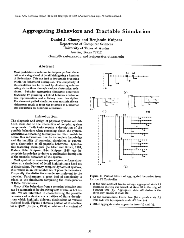
levels of detail. Figure 1 showsa portion of this lattice
for a QSIM[Kuipers, 1986] simulation of a variant of
(d)
Figure 1: Partial lattice of aggregated behavior trees
for the PI Controller
¯ In the most abstract tree (a, at top), aggregatedstate
abstracts the two waybranch at state B1 in the original
behavior tree (d). Aggregated state A2 abstracts the
three-way branch at state B2.
¯ At the intermediate levels, tree (b) expands state
from (a); tree (c) expandsstate A2from
¯ Other aggregate states appear in trees (b) and (c).
38
From: AAAI Technical Report FS-92-03. Copyright © 1992, AAAI (www.aaai.org). All rights reserved.
a Proportional Integral (PI) controller. The modeler
can move through this abstraction space and select a
description which highlights the distinctions of interest. The computational complexity of a qualitative
simulation is reduced and the resulting behavioral descriptions are simplified by eliminating uninteresting
details.
Techniques have been developed that allow the modeler to view the behavior of the system from various
perspectives and at various levels of abstraction. This
paper will discuss two of these methods:
Behavior aggregation observes similarities
between
states in the behavior tree. Similar behaviors are
combined into a single aggregate behavior during
simulation to eliminate occurrence branching. Occurrence branching is the complete temporal ordering of upcoming events whose order is not constrained by the QDE.This builds on work done by
Williams [1986] and Fouch~ and Kuipers [1991].
Envisionment guided simulation
initially performs an attainable envisionment. Various paths within the envisionment are then identified
and these paths are used as a guide when developing
a behavior tree.
In addition, Wood Wai Lee [1992] has developed a
method for abstracting infinite behaviors. A finite
structure is developed by observing regularities within
the behavior.
Qualitative
Simulation
Qualitative simulation techniques derive a behavioral
description of a physical device from a structural representation. Constraints are specified for a set of variables via a qualitative differential equation (QDE).
These variables are described by a set of qualitative
values each containing a qualitative magnitude and a
direction of change. The domain of each qualitative
magnitude is described by a quantity space which specifies a finite, totally ordered set of landmarkvalues. A
qualitative magnitude is either a landmark or an open
interval between landmarks. The simulation uses the
QDEto derive a qualitative description of the system
behavior.
A total envisionment, used in Forbus’ Qualitative Process Theory [Forbus, 1984] and deKleer and
Brown’s Confluences [de Kleer and Brown, 1984], describes all possible states of the system. The qualitative states are represented as nodes in a directed graph
with edges connecting temporally adjacent states. An
attainable envisionment contains the subgraph that is
reachable from an initial state.
QSIM[Kuipers, 1986] uses a tree of qualitative
states to represent the behaviors which follow from a
set of initial values. Each path through the behavior tree represents a different system behavior. New
landmarks are created during the simulation identifying newly discovered critical values within the quan-
tity spaces of the state variables. The behavior tree
representation along with the new landmarks are used
by behavior-based filters [Fouch~ and Kuipers, 1992,
Lee and Kuipers, 1988] to eliminate spurious behaviors from the tree. Semi-quantitative reasoning techniques
[Kuipers and Berleant, 1988,
Berleant and Kuipers, 1991, Kay and Kuipers, 1992]
provide a more detailed description of the behaviors
by inferring quantitative bounds for the newly introduced landmarks.
Williams [1986] describes an alternate simulation
technique based upon individual variable histories. A
history defines a sequence of qualitative values for a
single variable. A concise history is a sequence of such
values in which each value is distinct from its neighbors. The behavior of the system is described in terms
of a history for each variable. Histories are temporally
correlated only when necessary as opposed to the complete temporal ordering provided by a behavior tree or
envisionment representation.
These techniques for describing the behavior of a
system are effective in different situations. Our techniques integrate these three methods. Behavior aggregation provides a hybrid between a behavior tree
representation and a history based description, while
envisionment guided simulation begins with an envisionment graph before developing a limited behavior
tree.
Behavior
Aggregation
Behavior aggregation attempts to eliminate distinctions which do not affect the subsequent behavior of
the system. Figure 2 summarizes various abstraction techniques for envisionment graphs developed by
Fouch~ and Kuipers [1991]. Behavior aggregation extends their behavior based abstraction techniques to
other types of occurrence branching and performs the
aggregation on the fly (i.e. while the simulation is occurring) during a behavior tree simulation. Behavior
aggregation is being extended to include other abstraction techniques.
Occurrence branching results when the temporal ordering of a set of events is unconstrained by the QDE.
An event occurs when a variable crosses a landmark
or its derivative reaches zero. Following the events
that cause the occurrence branch, the behaviors return
to qualitatively equivalent states and the subsequent
behaviors are identical. This branching needlessly increases the complexity of the simulation and of the
behavior tree.
In its simplest form, occurrence branching results
when the events occur among unrelated variables. In
this case, the only qualitative distinction amongthe
behaviors is the temporal ordering of the events. In
more complicated instances, the variables are related
via a derivative relationship. Distinct histories result
when the occurrence branch involves a variable approaching a landmark while its derivative approaches
39
From: AAAI Technical Report FS-92-03. Copyright © 1992, AAAI (www.aaai.org). All rights reserved.
Fouch~ and Kuipers [1991] apply state-based
and
behavior-based
abstraction
techniques to attainable
envisionment graphs to provide a hierarchy of descriptions. A more abstract graph results with one state for
each equivalence class.
Twobehaviors (a) from branch B1 in figure ld showing
landmark attainment branch on -1 at time t4. In the first
behavior, the derivative reaches zero before the landmark
is attained while in the other behavior these two events
occur simultaneously. All other variables have identical
histories. An abstract state is formed at (t4 t5) when
the magnitudes are equivalent. The completed aggregate
behavior (b) eliminates landmark F-0 since it cannot
matched against a landmark in the other behavior. The
qualitative magnitude at t4 becomes [-1 0).
¯ The state based techniques eliminate distinctions
by
combining states into equivalence classes by focusing on
certain distinctions in the qualitative states.
Focus On:
Qualitative
Branches Eliminated:
Magnitude
Qualitative
Derivative
Interesting
Variables
Eliminates chatter except
around zero.
Some occurrence branching
Eliminates
distinctions caused by intermediate variables including
occurrence branching and
chatter within these variables.
¯ The behavior based abstraction method eliminates occurrence branching by collapsing Single Input Single Output (SISO) subgraphs within the envisionment
graph. All paths through the SISO subgraph must have
identical concise histories.
""’,t....~_.% ~
"i
techniques
from
zero. Once the derivative
reaches zero, the variable
no longer attains
the approaching landmark. This is
referred to as landmark attainment occurrence branching. Figure 3 describes two instances of this within the
PI-controller simulation.
,t,.~..~.,.4,.. 4.._4..,4._.4.
~ -r
.,,~..., 0
--’H-H-"
,
f(error)
Figure 2: Summary of abstraction
[Fouchd and Kuipers, 1991]
?
A~egete
°it""
9eb 2
(b)
¯ Three behaviors (c) from branch B2 in figure ld showing a landmark attainment branch on I-0 between t6 and
t8. The first behavior exceeds the landmark, the second
does not reach it while the third becomes steady at the
landmark. An abstract state is formed once the magnitude rises above I-0. The completed aggregate behavior
(d) eliminates landmarks I-5 and I-7 since they cannot
be matched. The qualitative
magnitude at t6 becomes
(minf 0).
Behavior aggregation eliminates occurrence branching by combining the behaviors in the resulting
subtree into a single aggregate state. An aggregate state
represents
an open time interval
which describes the
behavior of the system at various levels of detail using
individual histories
for each variable.
The temporal
correlation
between events is eliminated. The simulation is continued for this subtree from a single abstract
state.
Occurrence branching can occur at various points
throughout the simulation.
This results
in a lattice
of behavioral descriptions
depending upon which instances of occurrence branching are eliminated.
Figure 1 shows a portion of this lattice for the PI-controller
simulation.
The user can move through this abstraction space either manually or automatically to select
the appropriate level of description.
Behavior aggregation initially
performs the simulation at the highest
level of abstraction.
The more detailed levels of description
are only calculated
when requested by the
modeler. This lattice of descriptions
will be extended
further as more abstraction
techniques are developed.
I : integral (error) Aggregate Beh 2
(d)
Figure 3: Original
PI-controller
40
and aggregated
behaviors
for the
From: AAAI Technical Report FS-92-03. Copyright © 1992, AAAI (www.aaai.org). All rights reserved.
Aggregate States
An aggregate state describes a set of similar segments
of parallel behaviors. It abstracts the shared properties
of these behavior segments by using a history based description to characterize the behavior of each variable
independently. A hierarchy of descriptions is provided
allowing the modeler to view the histories at various
levels of detail.
History Graph The set of histories for each variable
can be combined into a graph with a single starting point and single ending point. Often, this combination results in a single unique concise history.
However, due to landmark attainment occurrence
branching, all of the histories for a single variable
are not necessarily identical (see figure 3).
A Single Aggregate History The history graph is
abstracted to a single concise history. The union of
the qualitative values at each branch in the history
graph is used to form this history. This history is
used in the standard QSIMbehavior display.
Summary Value A single qualitative
value which
provides an upper and lower bound for the histories over this interval. This level of description is
used by various filters within QSIM.
As other abstraction techniques are developed, the history graph will prove particularly useful since it allows
the modeler to view the behavior of each system variable independently. The only information that is lost
from the original behavioral description is the temporal
correlation between events in different variable histories.
The Algorithm
Behavior aggregation maintains a record of qualitatively equivalent states within the behavior tree.
Equivalent states are combined into a single abstract
state when they form a spanning set for a subtree
within the behavior tree. This subtree is collapsed
into an aggregate state and the simulation continues
from the abstract state. The four main steps within
the algorithm are:
1. Determining the qualitative equivalence of states.
2. Combiningequivalent states into a single abstract
state.
3. Selecting subtrees to aggregate.
4. Abstracting the subtree into an aggregate state.
Qualitative
Equivalence The QSIMalgorithm defines a qualitative state by a set of qualitative values
and a quantity space (qspace) for each state variable.
Twostates are considered qualitatively equivalent if
each variable has (1) the same qualitative magnitude
with respect to the joint qspace for that variable, and
(2) the same direction of change. The joint qspace for
a variable is defined as the intersection of the qspaces
for the states being compared. The joint qspace eliminates any landmarks which have been introduced since
these behaviors diverged.
Combining Equivalent States Behavior aggregation combinesqualitatively equivalent states into a single minimally abstract state. The quantity space for
each variable is constructed by combining the qspaces
from the equivalent states.
Landmarks which have
been introduced since the behaviors diverged must either be matched against equivalent landmarks in the
other states or eliminated. The qualitative values in
the abstract state are defined over these new quantity
spaces.
A minimally abstract state matches as many landmarks as possible thereby minimizing the number of
eliminated landmarks. Two landmarks can be matched
if they are defined within the sameinterval of the joint
qspace and have been created for the same reason.
Landmarksare created for various reasons including region transitions and changes in the direction of change.
Figure 3 demonstrates the elimination of landmarks
from the abstract state. Following the creation of an
aggregate state, the simulation will be continued from
this minimally abstract state.
Selecting
Subtrees for Aggregation
Behaviors
within a tree can be combinedin various ways to highlight different distinctions. Currently, behavior aggregation is applied whena set of qualitatively equivalent
states form a spanning set for a subtree within the behavior tree. A spanning set must contain one state
from each path in the subtree. Methods of loosening
this restriction are currently being investigated. The
behavior segments extending from the root of the subtree to the spanning set are combinedinto an aggregate
state.
Aggregating a Subtree A single aggregate state is
formed from the selected subtree. An aggregate state
uses a history based approach to describe the behavior
of each system variable over the abstracted time interval. For each variable a set of concise histories defined
over the same quantity space is derived from the behavior tree. For most variables these concise histories
will be identical. The concise histories are combined
into a history graph with a single beginning point and a
single ending point. Each history graph is summarized
by a single aggregate history which eliminates branching by using a more abstract qualitative description.
The most abstract description of the behavior by an
aggregate state consists of a single summaryvalue for
each variable. The summaryvalue is the union of the
values taken on by that variable in its history.
The spanning set algorithm generalizes and extends
the Single-Input Single-Output (SISO) subgraph used
by Fouch~ and Kuipers [1991]. The states that com-
41
From: AAAI Technical Report FS-92-03. Copyright © 1992, AAAI (www.aaai.org). All rights reserved.
prise the spanning set are represented by a single state
in an envisionment graph. Whenthey are combined
into an abstract state, a SISO subgraph is formed in
the behavior tree. This subgraph is then collapsed
into an aggregate state. Fouch~ and Kuipers require
all paths within the SISO subgraph to have identical
concise histories for the abstraction to be performed.
This restriction is eliminated in behavior aggregation.
In addition, behavior aggregation is performed on the
fly during a behavior tree simulation. It reduces the
complexity of the simulation while allowing for the introduction of new landmarks and the application of
behavior-based filters.
Envisionment
Guided
Simulation
Large models of dynamical systems often result in
intractable simulations and extremely large behavior
trees. Frequently, only a portion of the system behavior is of interest to the modeler at any one time. In
a complexbehavior tree, it is difficult to isolate and
analyze the particular behaviors of interest due to the
proliferation of states.
An attainable envisionment provides a more concise, finite representation of the behavior. Each path
through the graph represents a different behavior.
While the description is finite, many of the behaviors entailed by an envisionment graph are spurious
and are not true behaviors of the physical system. As
discussed earlier, one of the advantages of a QSIMbehavior tree simulation is the introduction of landmarks
throughout the simulation. Various behavior based
filtering techniques use these landmarks to eliminate
spurious behaviors and obtain more information about
the simulation. These filtering techniques include
the energy constraint [Fouch~ and Kuipers, 1992], the
non-intersection constraint [Lee and Kuipers, 1988],
and semi-quantitative
reasoning methods such aa
Q2, Q3 and NSIM. [Kuipers and Berleant,
1988,
Berleant and Kuipers, 1991, Kay and Kuipers, 1992].
Envisionment guided simulation uses an attainable
envisionment graph to focus the attention of the behavior tree simulation on the behaviors of interest. Figure 4 shows howthis can result in a tractable simulation of a portion of the behavior tree. The behavior
tree simulation uses a subgraph within the attainable
envisionment as a guide during simulation. Only those
behaviors that lie completely within the selected subgraph are simulated and included in the behavior tree.
This allows the modeler to eliminate intractable portions of the behavior tree from the simulation. It reduces the complexity of the behavior tree simulation
while retaining the behavior based filters and the ability to characterize the system behavior through the
introduction of landmarks.
Paths through the envisionment graph are selected
to form the subgraph used as a guide during the behavior tree simulation. A boolean expression can be
used to automatically select these paths. The expres-
b
(a)
(b)
-iI
i
,
"...~-.,~r--q--4"*
-z 3
°c~s
O: IZ’Z:O~ ]JQh I
(~)
¯ The spanning graph of the attainable envisionment (a)
contains 9 behaviors. A complete behavior tree simulation (figure ld) results in intractable branching.
¯ Thecyclic behavior (behavior 3) is selected for an envisionment guided simulation. Behavior aggregation eliminates an occurrence branch and a single behavior (b)
results. The QSIMenergy constraint is used to identify
the cycle as a decreasingoscillation (c).
Figure 4: An envisionment guided simulation of the PI
Controller demonstratinl~ a decreasing oscillation.
sion specifies conditions on the qualitative values of
states or sequences of states. All paths that satisfy
these conditions are selected. Subgraphs can also be
identified by selecting behavior numbers from the display or manually entering a list of paths through the
graph.
Envisionment guided simulation maintains a mapping between states in the envisionment subgraph and
their refinements in the behavior tree. A behavior tree
state provides a more detailed description of the system due to the introduction of new landmarks. The
refinement relation requires the qualitative values of
the behavior tree state to be equal to or more detailed
than those of the envisionment state. Only states that
provide a refinement of an envisionment state along
the traversed path are retained in the behavior tree.
Figure 5 demonstrates this filtering technique.
The resulting behavior tree is a refinement of the
identified envisionment subgraph. Uninteresting behaviors are eliminated and standard QSIMtechniques
are used to provide a detailed description of the desired
behaviors.
Conclusions
Qualitative reasoning techniques provide a mechanism
for reasoning from incomplete knowledgeabout the set
of possible behaviors of a physical system. These tech-
42
From: AAAI Technical Report FS-92-03. Copyright © 1992, AAAI (www.aaai.org). All rights reserved.
versity of Texas at Austin. Research of the Qualitative
Reasoning Group is supported in part by NSFgrants IRI8905494, IRI-8904454, and IRI-9017047, and by NASA
contract NCC2-760. Thanks to AdamFarquhar for help in
developing the envisionmentguided simulation algorithm.
E4
~E
3//~sionme~t
Subgraph
References
D. Berleant and B. J. Kulpers. Bridging the gap from
qualitative to numerical simulation. Technical Report
AI91-158,Artificial Intelligence Laboratory,University of
Texas at Austin, Austin, Texas 78712, Maxch1991.
J. de Kleer and J. S. Brown.A qualitative physics based
on confluences.Artificial Intelligence, 24:7-83, 1984.
B. Falkenheiner and K. D. Forbus. Setting up laxge-scale
qualitative models. In Proceedingsof the Seventh National
Conference on Artificial Intelligence (AAAL88), pages
301-306,, 1988.
K. D. Forbus. Qualitative process theory. Artificial Intelligence, 24:85-168,1984.
P. Fouch~and B. J. Kuipers. Towards a Unified Framework for Qualitative Simulation. In Proceedings of the
Fifth International Workshopon Qualitative Reasoning
about Physical Systems, 295-301, 1991.
P. Fouch~and B. J. Kuipers. Reasoning about energy in
qualitative simulation. In IEEETransactions on Systems,
Manand Cybernetics, 22, 1992.
H. Kay and B. J. Kuipers. Numerical Behavior Envelopes
for Qualitative ModelsIn Proceedingsof the Sixth International Workshopon Qualitative Reasoning, 1992.
B. J. Kulpers and D. Berleant. Using incomplete quantitative knowledgein qualitative reasoning. In Proceedings
of the Seventh National Conferenceon Artificial Intelligence, pages 324-329, 1988.
B. J. Kuipers. Commonsense
reasoning about causality :
Deriving behavior from structure. Artificial Intelligence,
24:169-204, 1984.
B. J. Knipers. Qualitative simulation. Artificial Intelligence, 29:289-338, September1986.
W. W. Lee. A Qualitative Simulation Based Approach to
AutomateConstruction of Phase Portraits. Ph.D. diss.,
Dept. of ComputerScience, Univ. of Texas. Forthcoming.
W. W.Lee and B. J. Kuipers. NonIntersection of Trajectories in Qualitative Phase Space: A Global Constraint
for Qualitative Simulation. In Proceedings of AAAI 88,
286-291, 1988.
B. C. Williams. Doingtime: Putting qualitative reasoning
on firmer ground. In Proceedingsof the AmericanConference on Artificial Intelligence (AAAI’86),pages 105-113,
Philadelphia, PA. August1986.
refinment
relation
$2
BehaviorTree
$1 in the behavior tree is a refinement of E1 in the envislonment subgraph. $2 is a possible successor to $1. $2 is
retained in the behavior tree if one of the followingconditions is met:
¯ E1 is a time intervMstate and $2 is a refinementof El.
¯ $2 is a refinement of either E2 or E3.
$2 is suspendedfromfurther simulationif it does not satisfy
one of these conditions. Multiple behavior tree states may
mapto the same envisionment graph time interval state
due to the introduction of landmarksin the behavior tree.
Figure 5: Development of the behavior tree using envisionment guided simulation
niques can be used in a number of tasks including diagnosis, design, explanation, and question answering.
Qualitative reasoning techniques, however, tend to reason at a single level of abstraction. This can lead to
a large number of possible behaviors and a possibly
intractable simulation.
Behavior aggregation limits the complexity of the
qualitative simulation by combining similar behaviors
to eliminate occurrence branching. Other abstraction
techniques are being developed to further reduce the
complexity of the qualitative simulation. These include
techniques to automatically eliminate chatter while a
behavior tree simulation is being performed. In addition, static evaluation methods are being investigated
which identify loosely connected components within
the QDE.The simulation of these components can be
performed independently and combined only when the
components interact.
Envisionment guided simulation allows the modeler
to perform a limited behavior tree simulation focusing attention on selected behaviors and eliminating
intractable branches. The complexity of the simulation depends upon the selected behaviors. Thus, intractable branches which are not of interest are eliminated from the simulation.
Acknowledgments
This work has taken place in the Qualitative Reasoning
Groupat the Artificial Intelligence Laboratory, The Uni-
43


