A Hybrid Model for Situation Monitoring and Conflict Prediction in Human
Supervised “Autonomous” Systems
Charles Lesire and Catherine Tessier
ENSAE-Supaero, Toulouse, France
Onera-DCSD, Toulouse , France
{lesire,tessier}@onera.fr
Abstract
The paper focuses on a key issue for human supervised “autonomous” systems, namely situation monitoring. The operator’s involvement within human-robot team is first described
as the way they close the control and decision loops. Then a
framework based on particle filtering and Petri nets is presented for hybrid numerical-symbolic situation monitoring
and inconsistency and conflict prediction within the team.
Human-robot team and the operator’s
involvement
Autonomy is not an end in itself in robotic systems. Autonomy is needed because we want robots to be able to cope
with mission hazards when communications with the human
operator are impossible (due to communication gaps, discretion requirements, or to the operator’s workload). Therefore adjustable autonomy must be considered to enable the
robots to compensate for the operator’s neglect (Goodrich et
al. 2001). The control of shared autonomy may be humaninitiated, a priori scripted or robot-initiated (Brookshire,
Singh, & Simmons 2004). Whatever the case, implementing
adjustable autonomy requires situation awareness (Endsley
2000) – including predicting what is likely to happen next –
both from the operator’s and robot’s points of view (Drury,
Scholtz, & Yanco 2003).
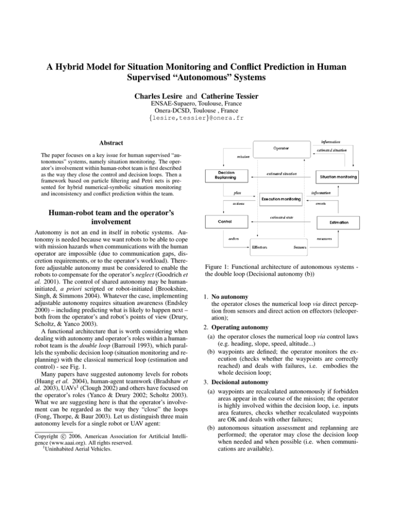
A functional architecture that is worth considering when
dealing with autonomy and operator’s roles within a humanrobot team is the double loop (Barrouil 1993), which parallels the symbolic decision loop (situation monitoring and replanning) with the classical numerical loop (estimation and
control) - see Fig. 1.
Many papers have suggested autonomy levels for robots
(Huang et al. 2004), human-agent teamwork (Bradshaw et
al. 2003), UAVs1 (Clough 2002) and others have focused on
the operator’s roles (Yanco & Drury 2002; Scholtz 2003).
What we are suggesting here is that the operator’s involvement can be regarded as the way they “close” the loops
(Fong, Thorpe, & Baur 2003). Let us distinguish three main
autonomy levels for a single robot or UAV agent:
c 2006, American Association for Artificial IntelliCopyright gence (www.aaai.org). All rights reserved.
1
Uninhabited Aerial Vehicles.
Figure 1: Functional architecture of autonomous systems the double loop (Decisional autonomy (b))
1. No autonomy
the operator closes the numerical loop via direct perception from sensors and direct action on effectors (teleoperation);
2. Operating autonomy
(a) the operator closes the numerical loop via control laws
(e.g. heading, slope, speed, altitude...)
(b) waypoints are defined; the operator monitors the execution (checks whether the waypoints are correctly
reached) and deals with failures, i.e. embodies the
whole decision loop;
3. Decisional autonomy
(a) waypoints are recalculated autonomously if forbidden
areas appear in the course of the mission; the operator
is highly involved within the decision loop, i.e. inputs
area features, checks whether recalculated waypoints
are OK and deals with other failures;
(b) autonomous situation assessment and replanning are
performed; the operator may close the decision loop
when needed and when possible (i.e. when communications are available).
Remark 1 The operator closes the numerical or decision
loop provided required communications with the robot are
available.
Remark 2 In case of emergency, a manual handover may
be possible (provided required communications are available).
Situation monitoring is a key issue in human-robot teams:
indeed situation monitoring has to maintain both the operator’s situation awareness and situation assessment for the
robot (Drury, Scholtz, & Yanco 2003), so that the task context should not be lost when the robot cedes control to the
human or conversely (Brookshire, Singh, & Simmons 2004).
What is more is that the global human-robot team must be
predictible whatever may occur, e.g. failures, operator’s
omissions or wrong moves. Therefore what is needed is
a global situation monitoring to track and predict the behaviour of the human-robot team, according to the human’s
involvement into the control loops, and possibly detect inconsistencies within the team.
As it is already clear with the double-loop representation
(see Fig. 1), human-robot team are hybrid systems, in so
far as both numerical (continuous) and symbolic (discrete)
parts are involved. It must be noticed that the discrete part
is not a mere abstraction of the continuous part - as it is
the case in most of the hybrid system literature: indeed
the discrete part mostly corresponds to how the operator
interacts with the robot and sets configurations or modes.
What is presented in the paper is a way to estimate and
predict the states in such hybrid systems through a unified
model, and how conflicts (possibly leading to dangerous
situations) may be predicted within the team.
After an overview of hybrid system estimation methods,
the particle Petri net - a joint model for situation monitoring in hybrid systems - will be presented. Afterwards the
estimation principles will be described and illustrated on the
thermostat example. Finally the application of particle Petri
net-based estimation to situation monitoring in human supervised “autonomous” systems will be dealt with.
Hybrid State Estimation
Estimating the state of a hybrid system is widely studied
in the literature and involves a large amount of techniques,
from numerical filters to network models.
In (Veeraraghavan & Papanikolopoulos 2004) the estimation rests on a set of Kalman filters, each one tracking a linear mode of the system. The most probable states allow to
determine the most probable filter and then the most probable mode of the system (i.e. the most probable behavior
of a car like turning, accelerating, etc.) In the same way,
(Koutsoukos, Kurien, & Zhao 2003) propose an estimator
based both on hybrid automata to represent the mode evolution and on a particle filter to estimate the continuous state
of the system. The estimated mode is then the most probable
mode of the system with respect to the estimated continuous
states. A similar principle is applied in (Hofbaur & Williams
2002) who use a concurrent probabilistic hybrid automaton
(cPHA) to estimate the mode of the system using Kalman
filters.
Bayesian networks are also used to represent hybrid systems by modeling the links between discrete and continuous variables in terms of conditional probabilities over time.
Inference rules (Lerner & Parr 2001) or particle filtering
(Doucet et al. 2000) can be used to estimate the state of
a hybrid system. However Bayesian networks suffer from:
1. the necessity to define a measure (probability, possibility. . . ) on the (continuous and discrete) state. This is
sometimes impossible to do for instance in case of complete uncertainty (see (Chachoua & Pacholczyk 2000));
2. the fact that an analysis on the consistency of the discrete
and continuous states is difficult to perform as the estimations on discrete and continuous states are aggregated
within the probability distribution.
In the same way, the analysis of conflicts, or conversely
consistency, is mainly based on the study of continuous
variables. In (Benazera & Travé-Massuyès 2003) the hybrid
system must satisfy constraints that are checked on the
continuous estimated states of the system. (Del Vecchio
& Murray 2004) use lattices to identify the discrete mode
of a hybrid system when only continuous variables are
observed. In (Tomlin et al. 2003), the reachability analysis
of continuous states, based on hybrid automata, allows to
identify safe and dangerous behaviors of the system and is
applied to an aircraft collision problem. Nielsen and Jensen
(Nielsen & Jensen 2005) define a conflict measure on the
estimated state of a Bayesian network; nevertheless this
method still suffers from the need to define a measure on
totally uncertain states, and from the fact that the conflict
measure is continuous, which leads to a threshold effect.
In (Lesire & Tessier 2005) an aircraft procedure and pilot’s
actions are jointly modeled using a particle Petri net that
allows the procedure to be simulated using a Monte-Carlo
method and the results to be analysed using the Petri net
properties. Hence only the nominal procedure is modeled
and the analysis is based on qualitative properties and does
not involve any continuous measure.
The monitoring system presented in this paper is based on
the later work: it allows both the estimation to be computed
and the consistency of the estimated states to be analysed
without defining a priori measures on unknown states. Indeed it is the structure of the Petri net-based model itself
which allows the consistency to be checked. The next section mentions the main definitions of particle Petri nets.
Particle Petri Nets
Prerequisites
Particle Filtering The particle filter (Arulampalam et al.
2002) allows the state xk at time k of a dynamic system subject to deterministic and random inputs to be estimated from
observations zk spoilt with stochastic errors. It is based on a
discretization of the uncertainty on the state value: the probability distribution function of the estimate x̂k|k – meaning
the state estimated at time k knowing the observation at time
(1)
(N )
k – is represented by a set of N particles xk|k , . . . , xk|k (see
Fig. 2). The estimation is achieved through a two-step process : the prediction, that consists of estimating the next
(i)
particles xk+1|k according to the evolution model, and the
correction, that is based on a comparison of the expected
particle values with the observation: the closer the expected
particles are to the most probable value of the observation,
the bigger weight they are assigned. Then N new particles
(i)
xk+1|k+1 are generated from a resampling of the weighted
corrected particles.
numerical and symbolic transitions allow all the expected
states of the system to be computed whatever the actions.
Figure 3 is the particle Petri net of a thermostat. The thermostat manages temperature2 θ between 20◦ C and 25◦ C.
The numerical places p0 , p1 and p2 are associated with differential equations modeling heating (θ̇ = −0.2θ + 5.4) and
cooling (θ̇ = −0.1θ +1.2) respectively. The numerical transitions correspond to guards: transitions θ > 25 and θ < 20
indicate respectively that the temperature is and is not warm
enough. The symbolic places indicate the modes of the thermostat (on or off) and the symbolic transitions (OF F ) represent external actions to turn off the thermostat.
Figure 2: Particle filtering (from (Lehmann 2003))
Petri Nets A Petri net < P, T, F, B > is a bipartite graph
with two types of nodes: P is a finite set of places; T
is a finite set of transitions (David & Alla 2005). Arcs
are directed and represent the forward incidence function
F : P × T → N and the backward incidence function
B : P × T → N respectively. An interpreted Petri net is
such that conditions and events are associated with places
and transitions. When the conditions corresponding to some
places are satisfied, tokens are assigned to those places and
the net is said to be marked. The evolution of tokens within
the net follows transition firing rules. Petri nets allow sequencing, parallelism and synchronization to be easily represented.
Particle Petri Nets
A particle Petri net (Lesire & Tessier 2005) is a hybrid Petri
net model where places and transitions are either numerical
or symbolic:
1. numerical places PN are associated with differential
equations representing the continuous evolution of the
system;
2. numerical transitions TN are associated with conditions
and represent mode changes in the system dynamics;
3. symbolic places PS and transitions TS are associated with
symbolic states and actions respectively.
The state of the system is represented by a set of tokens,
(i)
that are particles πk+1|k – meaning particle number i at
time k + 1 knowing the observation at time k –, evolving
within the numerical places, and a set of configurations
(j)
δk+1|k evolving within symbolic places.
A marking
mi,j = (π (i) , δ (j) ) represents a possible state of the system.
The firing rules (Lesire & Tessier 2005) associated with
Figure 3: The thermostat particle Petri net
Estimation principles
The estimator presented here is based on the particle filtering
principle and computes the expected markings of a particle
Petri net. The estimation is achieved through a two-step process:
1. a prediction of the expected markings, according to the
particle Petri net firing rules, that computes all the possible combinations of numerical and symbolic states;
2. a correction of the markings according to an observation
made on the system.
Prediction
The prediction is achieved through the computation of the
reachable markings of the particle Petri net, i.e. the set of the
expected states. It is based both on an isoparticle evolution,
i.e. an evolution of the tokens within the net to model mode
changes according to actions, and an isomarking evolution,
i.e. an evolution of the particles according to differential
equations.
Let us consider the example of the thermostat (Fig. 3),
(0)
and let the initial marking be π0|0 = 20◦ C marking place
p0 and δ (0) marking place on. Then the expected marking at
time 1 is the marking shown on Fig. 4, where
1. in place p0 , particle π (0) = 21.4◦ C has evolved according
to the heating differential equation;
2
The temperature is noted θ in the text and T on figures as the
θ character is not available in the estimation software and T is already the set of transitions of the particle Petri net.
2. in place p2 , particle π (1) = 19.2◦ C has evolved according to the cooling differential equation, predicting the situation corresponding to the thermostat being turned off;
3. configurations δ (0) and δ (1) in symbolic places on and off
respectively indicate that the thermostat may be either on
or off at time 1.
of the data to be analysed. (2) means that particles π (i)
and π (j) are equivalent if they mark the same place p and
for each particle π (k) which is not in p, both π (i) and π (j)
have either a higher or lower weight than π (k) .
Remark 4 The algorithm applying recursively relation
R on particles and then on equivalence classes terminates
and computes at most N steps, where N is the number of
particles (the worst case considers that at each step only
two classes are equivalent).
3. updates (Benferhat, Lagrue, & Papini 2005) the ranking
of predicted configurations δk+1|k according to the observation. This results in a ranking of corrected configurations δk+1|k+1 (≺∆ means “is preferred to”):
(i)
(j)
(i)
(j)
(zk+1 →δk+1|k )∧(zk+1 6→δk+1|k )⇒δk+1|k+1 ≺∆ δk+1|k+1
where z → δ means that configuration δ matches observation z (see Example 1 below). (4) means that the configurations matching the observation are preferred to the
configurations not matching the observation.
Figure 4: Predicted marking at time 1
Thereby the marking at time k represents the estimated
states as a set of tokens – the set of particles being a discretization of the probability distribution on the continuous
state –, and the prediction step computes the expected marking at time k + 1.
(i)
(j)
If both δk+1|k and δk+1|k match (or do not match) the observation, the ranking is not changed, the relation between
(i)
(j)
(i)
δk+1|k+1 and δk+1|k+1 is the same as between δk+1|k and
(j)
δk+1|k :
(i)
(j)
(zk+1 →δk+1|k ∧ zk+1 →δk+1|k )
Correction
(i)
1. weights the predicted particles according to the noisy observation:
(1)
where zk+1 is the observation at time k + 1, w(π) is
the weight of particle π and p(z|π) is the conditional
probability to observe z knowing the expected state π;
2. groups the weighted particles according to the equivalence relation R:
8
(i)
(j)
>
>
< ∀p∈PN ,(π ∈M(p)⇔π ∈M(p))
(k)
(i)
π (i) Rπ (j) ⇔
∀π ∈Π / ∀p∈PN (π ∈M(p)⇒π (k) 6∈M(p)),
>
>
:
(w(π (i) )≥w(π (k) )⇔w(π (j) )≥w(π (k) ))
(2)
where Π = {π (i) , i ∈ J1; N K} and M(p) is the
marking of place p. The equivalence classes are noted
(i)
Γ = {γk+1|k }, and their weights are defined by
(i)
w(γk+1|k )=
P
π∈γ
(i)
k+1|k
w(π)
(3)
The process is then recursively applied on Γ to group the
equivalence classes until they are restricted to singletons;
Remark 3 The equivalence relation R is designed to
help diagnose the state of the system by reducing the size
(j)
(i)
(j)
(5)
(j)
(i)
(j)
(6)
⇒(δk+1|k+1 -∆ δk+1|k+1 ⇔δk+1|k -∆ δk+1|k )
The correction consists in comparing matchings between the
predicted tokens and the incoming observation and selecting
the “best” ones. The correction process:
(i)
p(zk+1 |π
)
(i)
k+1|k
w(πk+1|k )= PN
(j)
p(z
|π
)
k+1
j=0
k+1|k
(4)
(i)
(j)
(zk+1 6→δk+1|k ∧ zk+1 6→δk+1|k )
(i)
⇒(δk+1|k+1 -∆ δk+1|k+1 ⇔δk+1|k -∆ δk+1|k )
The relation -∆ (meaning “is preferred or equivalent to”)
is a partial preorder on the set of configurations;
Example 1 In the thermostat example, relation →, representing the matching between predicted configurations
and the observation, is defined by :
(a)
(b)
(c)
(d)
on → on and on 6→ off,
off → off and off 6→ on,
on ∧ off → on and on ∧ off → off
false → on and false → off
where case (c) corresponds to an observation of both
modes on and off, that may come from a sensor error, and
case (d) corresponds to an empty observation (false) that
may come from a sensor failure.
4. constructs the correction graph by ranking (relation -)
the markings mi,j = (γ (i) , δ (j) ), according to the weights
on γ (i) and to relation -∆ on configurations δ (j) :
(
mi,j ≺mk,l
⇔
mi,j ∼mk,l
⇔
w(γ (i) )≥w(γ (k) )∧δ (j) -∆ δ (l)
w(γ (i) )>w(γ (k) )∨δ (j) ≺∆ δ (l)
( w(γ (i) )=w(γ (k) )∧δ (j) ∼∆ δ (l) )
(7)
(8)
(i)
5. resamples the particles : N new particles πk+1|k+1
are drawn from the discrete probability law
(i)
(i)
{πk+1|k , w(πk+1|k )}.
The particles are then spoilt
with the model noise to represent the model approximation.
The resampled particles represent the estimated numerical states of the system at time k + 1 and are introduced
in the next prediction step. The correction graph built from
predicted tokens is analysed to detect inconsistencies. This
analysis is presented in the next section. The whole estimation process is illustrated through the thermostat example.
Consistency Analysis and Conflict Detection
A state of the system is said to be consistent if it is a possible
state with respect to the initial state and to the model of the
nominal behavior of the system. The set of possible states
can be computed before the on-line estimation and consists
in computing the reachable states of the particle Petri net.
Hence an ordinary safe Petri net4 is associated with the
particle Petri net of the system such as one ordinary token
is associated to each place corresponding to a marked (by
particles or by configurations) place in the particle Petri net.
Let the initial marking of the ordinary safe Petri net of the
thermostat (Fig. 3) be M0 = (1 0 0 1 0): places p0 and on
are marked, places p1 , p2 and off are empty. Then marking
M0 represents the initial state of the Petri net: the thermostat is on and heating.
The reachable states of the particle Petri net correspond
to the reachable markings of the safe Petri net represented
in Fig. 5. The graph of reachable markings is the classical
automaton of a thermostat, with three modes: on (marking
M0 ), idle (marking M1 ) and off (marking M2 ). Consequently the markings that are inconsistent in the estimation
process are:
1. M4 = (0 0 1 1 0), meaning that the thermostat is on but
the temperature decreases;
2. M5 = (1 0 0 0 1), meaning that the thermostat is off but
is still heating;
3. M6 = (0 1 0 0 1), meaning that the thermostat is off but
will heat as soon as the temperature is under 20.
Figure 5: Reachable markings of the thermostat Petri net
Remark 5 The computation of the reachable markings may
be complex in general as the set of reachable markings may
be infinite. Nevertheless the set of reachable markings of a
safe Petri net is finite.
4
An ordinary Petri net is a Petri net with no interpretation containing undifferentiated classical tokens. A Petri net is said to be
safe for an initial marking M0 if for all reachable markings, each
place contains zero or one token.
The consistency analysis is achieved through the study
of the correction graph computed during the correction process:
1. Each marking mi,j = (γ (i) , δ (j) ) is associated with a
marking m
e i,j in the associated safe Petri net:
(
∀p∈P =PN ∪PS ,
m
e i,j (p)=
if γ (i) ∈M(p)5 or δ(j) ∈M(p)
0 otherwise
1
2. Then the consistency of mi,j is checked:
mi,j is consistent ⇔ m
e i,j ∈ G
(10)
where G is the graph of the reachable markings of the safe
Petri net.
Knowing the (in)consistent markings of the correction
graph is a first step towards the detection of conflictual situations. Some issues in analysing such a graph are currently
under study, for instance about using the graph in the resampling strategy or identifying patterns in the correction graph
to detect well-known conflictual situations.
The next section presents some examples and results
about the estimation principle and the consistency analysis.
Simulations
Thermostat Monitoring
The initial marking of the thermostat is represented in Fig. 6
where 50 particles have been drawn from the normal distribution N (22◦ C, 1) – 22◦ C is the initially observed temperature.
Figure 6: Initial estimated state of the thermostat: the thermostat is on, heating, and the temperature is approximatively 22◦ C.
Temperature Estimation Figure 7 is the result of the estimation process launched on the Petri net of Fig. 6 with a
new observation of the temperature and the thermostat mode
every second. The dashed line represents the (noisy) observations and the crosses are the particles.
We can notice that the shape of the estimated temperature
smoothly fits the observed temperature, meaning that the estimation well corresponds to the thermostat behavior. To illustrate the estimation process, let us consider the correction
step at time 1.
By abuse of notation, γ (i) ∈ M(p) means that all the particles
in γ are marking place p (which is true by construction of γ (i) ).
5
(i)
(9)
Figure 8: Correction graph at time 1
Figure 7: Estimation of the temperature
particle number
11
12
25
41
17
18
8
29
1
42
θ
21.581
21.594
21.535
21.615
21.618
21.624
21.630
21.502
21.638
21.642
weight
0.0361
0.0360
0.0360
0.0357
0.0357
0.0355
0.0354
0.0353
0.0352
0.0351
place
p2
p0
p0
p2
p0
p2
p0
p0
p0
p0
Table 1: Best weighted particles at time 1
The observation at time 1 is z1 = (21.567◦ C, on). Table 1
contains the ten best predicted particles according to z1 and
their associated weights. As far as the consistency analysis
is concerned, it is easily guessed that analysing the whole
table, containing fifty columns (one per particle), is not obvious. Then the particles are grouped in equivalence classes
according to relation R applied recursively: when the particles are ranked by weight, (2) consists in making classes by
grouping the particles by place following the ranking. The
first step of the construction results in the following equivalence classes:
1. γ (1) = {π (11) } with weight 0.0361 in p2 ,
2. γ (2) = {π (12) , π (25) , π (17) } with weight 0.1077 in p0 ,
3. γ (3) = {π (41) , π (18) } with weight 0.0702 in p2 ,
4. γ (4) = {π (8) , π (29) , π (1) , π (42) } with weight 0.1410 in
p0 .
Relation (2) applied recursively on
Γ = {γ (1) , γ (2) , γ (3) , γ (4) } gives as a final result:
1. γ (5) = {γ (4) , γ (2) } with weight 0.2487 in p0 ,
2. γ (6) = {γ (3) , γ (1) } with weight 0.1063 in p2 .
The associated correction graph is drawn in Fig. 8 where
δ (0) = on and δ (1) = off: as the observation is on, δ (0) ≺
δ (1) , and as w(γ (5) ) > w(γ (6) ), the marking relation is
m5,0 ≺ m5,1 , m5,0 ≺ m6,0 , m5,0 ≺ m6,1 , m5,1 ≺ m6,1
and m6,0 ≺ m6,1 .
The framed markings are consistent. As a result, the best
marking (the root of the graph) is consistent and matches the
on state (thermostat on and heating).
Inconsistent Behaviors In order to study the consistency
of the thermostat behavior, two faulty cases are considered.
Both consist in a wrong behavior of the thermostat that
stops heating at temperatures 26◦ C and 24◦ C respectively.
Case 1: Figure 9 is the result of the estimation of the thermostat that stops heating at 26◦ C. At time 7, the best
marking (given the observation at time 7) has a weight
of 0.9985 and matches the state idle (places p1 and on).
At time 8, the best marking has a weight of 0.9970 and
matches the state on (places p0 and on). The difficulty to
estimate the right state can be explained by the fact that
the behavior is misunderstood by the estimator as no particle has a temperature around 26◦ C. At time 22, the best
Figure 9: Conflict detection: the behavior of the thermostat
is unknown.
marking matches the idle state (place p1 and on) with a
weight of 1. Then from time 23, the best markings match
state off (places p2 and off) and consequently are inconsistent as the observation is on. The difficulty to track
the behavior results in the fact that the estimation is completely wrong: all the particles are out of the main part
of the Gaussian observation – 99% of the probability of a
Gaussian distribution is within [µ − 3σ; µ + 3σ] where µ
is the mean value and σ the standard deviation.
This case shows that the prediction does not match the
observations very well as nearly no particle has a temperature around 26◦ C. Nevertheless the estimation is able to
track the temperature over 25◦ C. Switching from consistent to inconsistent matchings (times 7 and 8) reveals an
inconsistent behavior.
Case 2: Figure 10(a) is the result of the estimation of the
thermostat that stops heating at 24◦ C. In that case the estimation is completely different: all the correction graphs
from time 4 are the same (Fig. 10(b), where γ (1) ∈ p2 ).
Indeed the numerical observations can be explained as
they match the particles within place p2 . However the
symbolic observation is on. Then the best corrected marking is inconsistent and reveals a fault: the temperature
evolves as if the thermostat was off.
have attributes APPR, Flaps1 and Gear. The particles have
attributes x, y, z (the 3-D coordinates of the UAV), s (the
speed) and h (the heading).
The estimation of the UAV position (x and y coordinates)
is represented in Fig. 12. The dashed lines represent the
nominal trajectory of the UAV and the dots represent the
estimated particles.
(a) Estimation of the temperature
(b)
Correction
graph
Figure 10: Conflict detection: the behavior of the thermostat
corresponds to the off mode.
Estimation of the UAV-Operator Activities
This section presents an application of the estimation principle to a human–UAV team. This could be easily generalized to any human–robot or human–system team involving procedures (e.g. the Water Recovery System (Martin,
Schreckenghost, & Bonasso 2004)). The considered mission
is modeled by the particle Petri net of Fig. 11 and consists of
an Approach from waypoint A to waypoint B where actions
are shared between the UAV and the operator.
(a) at time 0
(b) from time 10
Figure 12: Estimation of the UAV position
At time 0, the UAV position is quite uncertain: the initial
distribution is diffuse. The estimation becomes more precise
from time 10.
At time 220, some particles mark place p2 (the UAV may
be decelerating) but the main corrected state matches place
p1 : the UAV is still turning. At this time the observation
states that the APPR button is not pressed. The correction
graph at time 220 is shown in Fig. 13, with γ (i) ∈ pi for
i ∈ {1, 2} and δ (j) ∈ pj for j ∈ {3, 4, 5, 6, 7}.
Figure 13: Correction graph of the mission at time 220
Figure 11: The particle Petri net of the Survey mission
Numerical places and transitions represent the trajectory
of the UAV. The procedure consists of a descent (place p0 )
from waypoint A. At 7 NM from A (transition d(A)>7NM),
the UAV starts turning (place p1 ) and when intercepting
heading 144◦ (transition Heading>144), the UAV has
to perform a deceleration (place p2 ). At 4 NM from B
(transition d(B)<4NM), the Approach procedure is finished:
the next phase is the Landing procedure. The symbolic transitions correspond to operator or UAV actions: pressing the
APPR button (transition APPR while descending or turning)
is an operator’s action, setting flaps 1 and setting the gear
down (transitions Flaps1 and Gear while decelerating) are
autonomous actions of the UAV. Then the configurations
Marking m2,3 is close to the best marking (m1,3 ) and is
inconsistent: it has to be studied and tracked while estimating the system state. Indeed it allows to anticipate a possible
conflict that may occur if the APPR button is not pressed in
a near future. At time 230 most of the corrected particles are
in p2 and the APPR button has been pressed (according to
the observation): a safe state is recovered.
Conclusion
The particle Petri net-based estimation principle that is presented in this paper paves the way to the detection of inconsistent behaviors in systems subjected to discrete actions –
e.g. human actions in a human–robot team.
Ongoing work is focusing on the analysis of the correction
graph, and more specifically on inconsistent states. What is
considered is to study the dynamics of inconsistent states
within the correction graph while monitoring the system in
order to design an automatic monitoring agent for hybrid
systems that would allow an early detection of conflicts and
if necessary the possibility to change the autonomy/control
level of the robot/human agents to face dangerous situations
or communication loss.
Experiments are being prepared with the flight simulator
at Supaero in order to assess conflict detection in procedures
involving complex autopilot modes.
References
Arulampalam, S.; Maskell, S.; Gordon, N.; and Clapp,
T. 2002. A Tutorial on Particle Filters for Online
Nonlinear/Non-Gaussian Bayesian Tracking. IEEE Transactions on Signal Processing 50(2):174–188.
Barrouil, C. 1993. Planification et analyse d’échec. In Fargeon, C., and Quin, J.-P., eds., Robotique mobile. Teknea.
chapter 10.1, 275–288.
Benazera, E., and Travé-Massuyès, L. 2003. The consistency approach to the on-line prediction of hybrid system
configurations. In ADHS’03.
Benferhat, S.; Lagrue, S.; and Papini, O. 2005. Revision
of partially ordered information: axiomatisation, semantics
and iteration. In IJCAI’05.
Bradshaw, J.; Sierhuis, M.; Acquisti, A.; Feltovich, P.;
Hoffman, R.; Jeffers, R.; Prescott, D.; Suri, N.; Uszok, A.;
and van Hoof, R. 2003. Adjustable autonomy and humanagent teamwork in practice: an interim report on space applications. In Hexmoor, H.; Castelfranchi, C.; and Falcone,
R., eds., Agent Autonomy. Kluwer. chapter 11, 191–220.
Brookshire, J.; Singh, S.; and Simmons, R. 2004. Preliminary results in sliding autonomy for coordinated teams. In
Interaction between humans and autonomous systems over
extended operations, AAAI Spring Symposium, 127–132.
Chachoua, M., and Pacholczyk, D. 2000. A symbolic approach to uncertainty management. Applied Intelligence
13(3):265–283.
Clough, B. 2002. Metrics, Schmetrics! How the heck
do you determine a UAV’s autonomy anyway? In Performance Metrics for Intelligent Systems Workshop.
David, R., and Alla, H. 2005. Discrete, continuous, and
hybrid Petri nets. Springer.
Del Vecchio, D., and Murray, R. 2004. Discrete state
estimators for a class of hybrid systems on a lattice. In
HSCC’04.
Doucet, A.; de Freitas, N.; Murphy, K.; and Russell, S.
2000. Rao-Blackwellised particle filtering for dynamic
Bayesian networks. In UAI’00.
Drury, J.; Scholtz, J.; and Yanco, H. 2003. Awareness in
human-robot interactions. In IEEE Conference on Systems,
Man and Cybernetics.
Endsley, M. 2000. Theoretical underpinnings of situation
awareness: a critical review. In Endsley, M., and Garland,
D., eds., Situation awareness analysis and measurement.
Lawrence Erlbaum Associates.
Fong, T.; Thorpe, C.; and Baur, C. 2003. Robot, asker
of questions. Robotics and Autonomous Systems 42(34):235–243.
Goodrich, M.; Olsen, D.; Crandall, J.; and Palmer, T. 2001.
Experiments in adjustable autonomy. In IJCAI’01 Workshop on Autonomy, Delegation and Control: interacting
with autonomous agents.
Hofbaur, M., and Williams, B. 2002. Mode estimation of
probabilistic hybrid systems. In HSCC’02.
Huang, H.-M.; Messina, E.; Wade, R.; English, R.; Novak,
B.; and Albus, J. 2004. Autonomy measures for robots.
In Proceedings of the IMECE: International Mechanical
Engineering Congress.
Koutsoukos, X.; Kurien, J.; and Zhao, F. 2003. Estimation
of distributed hybrid systems using particle filtering methods. In HSCC’03.
Lehmann, E. 2003. Particle filter. Ph.D. Coursework, Australian National Unversity.
Lerner, U., and Parr, R. 2001. Inference in hybrid networks: theoretical limits and practical algorithms. In
UAI’01.
Lesire, C., and Tessier, C. 2005. Particle Petri nets for aircraft procedure monitoring under uncertainty. In ATPN’05.
Martin, C.; Schreckenghost, D.; and Bonasso, R. 2004.
Augmenting automated control software to interact with
multiple humans. In Interaction between Humans and Autonomous Systems over Extended Operation, AAAI Spring
Symposium.
Nielsen, T., and Jensen, F. 2005. Alert systems for production plants: a methodology based on conflict analysis. In
ECSQARU’05.
Scholtz, J. 2003. Theory and evaluation of human robot interactions. In HICSS’03, 36th Annual Hawaii International
Conference on System Sciences.
Tomlin, C.; Mitchell, I.; Bayen, A.; and Oishi, M. 2003.
Computational techniques for the verification of hybrid
systems. IEEE 91.
Veeraraghavan, H., and Papanikolopoulos, N. 2004. Combining multiple tracking modalities for vehicle tracking in
traffic intersections. In ICRA’04.
Yanco, H., and Drury, J. 2002. A taxonomy for humanrobot interaction. In AAAI’02 Fall Symposium on HumanRobot Interaction.