From: AAAI Technical Report SS-03-02. Compilation copyright © 2003, AAAI (www.aaai.org). All rights reserved.
Finding Building Blocks Through Eigenstructure Adaptation
Danica Wyatt1, Hod Lipson2
1
2
Physics Department
Mechanical & Aerospace Engineering and Computing & Information Science
Cornell University, Ithaca NY 14853, USA
hod.lipson@cornell.edu
Abstract
A fundamental aspect of many evolutionary approaches to
synthesis of complex systems is the need to compose atomic
elements into useful higher-level building blocks. However,
the ability of genetic algorithms to promote useful building
blocks is based critically on genetic linkage – the
assumption that functionally related alleles are also
arranged compactly on the genome. In many practical
problems, linkage is not known a priori or may change
dynamically. Here we propose that the problems’ Hessian
matrix reveals this linkage, and that an eigenstructure
analysis of the Hessian provides a transformation of the
problem to a space where first-order genetic linkage is
optimal. Genetic algorithms that dynamically transform the
problem space can operate much more efficiently. We
demonstrate the proposed approach on a real-valued
adaptation of Kaufmann’s NK landscapes.
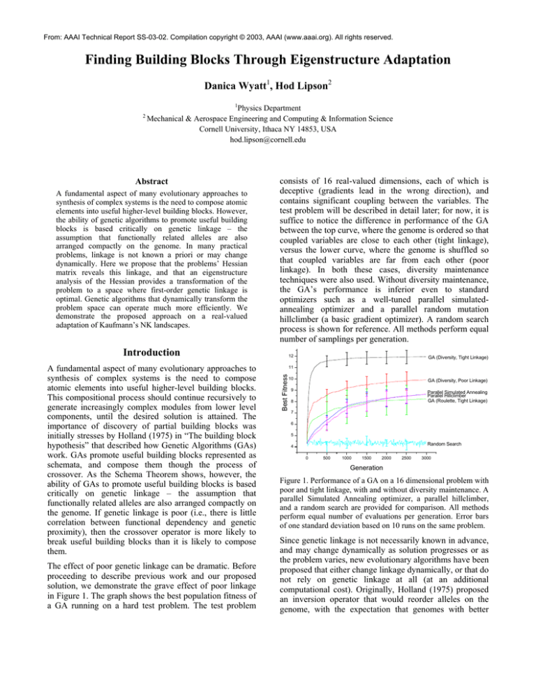
consists of 16 real-valued dimensions, each of which is
deceptive (gradients lead in the wrong direction), and
contains significant coupling between the variables. The
test problem will be described in detail later; for now, it is
suffice to notice the difference in performance of the GA
between the top curve, where the genome is ordered so that
coupled variables are close to each other (tight linkage),
versus the lower curve, where the genome is shuffled so
that coupled variables are far from each other (poor
linkage). In both these cases, diversity maintenance
techniques were also used. Without diversity maintenance,
the GA’s performance is inferior even to standard
optimizers such as a well-tuned parallel simulatedannealing optimizer and a parallel random mutation
hillclimber (a basic gradient optimizer). A random search
process is shown for reference. All methods perform equal
number of samplings per generation.
Introduction
The effect of poor genetic linkage can be dramatic. Before
proceeding to describe previous work and our proposed
solution, we demonstrate the grave effect of poor linkage
in Figure 1. The graph shows the best population fitness of
a GA running on a hard test problem. The test problem
GA (Diversity, Tight Linkage)
11
Best Fitness
A fundamental aspect of many evolutionary approaches to
synthesis of complex systems is the need to compose
atomic elements into useful higher-level building blocks.
This compositional process should continue recursively to
generate increasingly complex modules from lower level
components, until the desired solution is attained. The
importance of discovery of partial building blocks was
initially stresses by Holland (1975) in “The building block
hypothesis” that described how Genetic Algorithms (GAs)
work. GAs promote useful building blocks represented as
schemata, and compose them though the process of
crossover. As the Schema Theorem shows, however, the
ability of GAs to promote useful building blocks is based
critically on genetic linkage – the assumption that
functionally related alleles are also arranged compactly on
the genome. If genetic linkage is poor (i.e., there is little
correlation between functional dependency and genetic
proximity), then the crossover operator is more likely to
break useful building blocks than it is likely to compose
them.
12
10
GA (Diversity, Poor Linkage)
9
Parallel Simulated Annealing
Parallel Hillclimber
GA (Roulette, Tight Linkage)
8
7
6
5
Random Search
4
0
500
1000
1500
2000
2500
3000
Generation
Figure 1. Performance of a GA on a 16 dimensional problem with
poor and tight linkage, with and without diversity maintenance. A
parallel Simulated Annealing optimizer, a parallel hillclimber,
and a random search are provided for comparison. All methods
perform equal number of evaluations per generation. Error bars
of one standard deviation based on 10 runs on the same problem.
Since genetic linkage is not necessarily known in advance,
and may change dynamically as solution progresses or as
the problem varies, new evolutionary algorithms have been
proposed that either change linkage dynamically, or that do
not rely on genetic linkage at all (at an additional
computational cost). Originally, Holland (1975) proposed
an inversion operator that would reorder alleles on the
genome, with the expectation that genomes with better
orderings (tighter genetic linkage) would gradually take
over the population. However, this operator turned out to
be too slow in practice. A variety of algorithms were
proposed that do not assume linkage at all, and build up
the genome from scratch starting with the founding
building blocks. Goldberg et al (1989) developed the
Messy GA that evolves partial solutions in which allele
locations are moveable, and linkage can be adapted
through combination and split operators. Genetic
programming (Koza, 1989) combines building blocks in
tree hierarchies, allowing arbitrary branches of solutions to
be swapped and thereby permitting promotion of useful
subcomponents without relying on linkage (although GP is
usually applied to open-ended problems where linkage is
not well defined anyway). More recently, Harik and
Goldberg (1996) proposed a linkage learning genetic
algorithm (LLGA) that intersperses alleles in the partial
solutions with variable-sized gaps (introns) allowing the
GA more control over linkage tightening and exchange of
complete building blocks. A more recent version of this
algorithm uses evolved start expressions to assist in the
process of nucleation of tightly linked groups (Chen and
Goldberg, 2002). Watson and Pollack (2002) also coevolve partial solutions, but use symbiotic completion and
Pareto-dominance criteria to compare candidate
subcomponents, and assemble full solutions from scratch
without assuming linkage. The increased computational
cost comes through the exploration of many compositional
permutations offered by this formulation, but both of these
approaches have been shown to be able to synthesize
solutions to complex functions with multiple local optima,
which traditional GAs and gradient optimizers cannot
solve.
0
0
H =
2

0
0 2 0
0 0 3
0 0 0

3 0 0
(4)
Highly coupled variable pairs are represented by large
magnitude elements in H. Large, off-diagonal elements
imply coupling between variables that are not adjacent on
the genome; to improve linkage, variables can be
rearranged so that coupled pairs are proximate on the
genome, bringing their corresponding Hessian coefficient
closer to the diagonal. Rearranging the order of parameters
is equivalent to swapping rows and columns of H,
effectively transforming by a permutation transformation.
To bring the elements of H above closer to the diagonal
(effectively tightening the genetic linkage), we can use the
permutation matrix T, where
0
0
T =
1

0
1 0 0
0 1 0
0 0 0

0 0 1
(5)
to yield a new Hessian H’,
0
2
H ' = T T HT = 
0

0
2 0 0
0 0 0
0 0 3

0 3 0
and the improved genome ordering X’
X ' = XT = {x 3 , x1 , x 2 , x 4 }
Identifying linkage through the Hessian
Here we propose an alternative way of identifying building
blocks through dynamic eigenstructure analysis of the
problem landscape’s Hessian matrix. The matrix H is
defined by measuring the cross-correlation effect of the
variation of each of the n variables xi on the variation
effect of each other locus of the genome on the fitness
function F(X). Essentially, the Hessian matrix determines
the first-order functional dependencies between gene
locations. The Hessian is defined as
H ij =
∂F ( X ) 2
∂x i ∂x j
(1)
By definition, it is a symmetric matrix. For example, if
X=(x1, x2, x3, x4),
(2)
and the fitness function to be optimized is
F(X)=sin(2x1x3)+sin(3x2x4),
(3)
then computing H and evaluating at X=0 would yield
(6)
(7)
H’ above is as close as we can bring the non-zero elements
to the diagonal by reordering, and the resulting genome
ordering of Eq. (7) has indeed improved its linkage
compared to the original ordering of Eq. (2). But is there a
way to bring them even closer to the diagonal?
Generalized genome reordering
The optimal linkage ordering is not necessarily sequential.
In the example above, the permutation matrix simply
reorders elements on the genome. However, there might
not be a perfect sequential ordering if variables are coupled
in any way but a linear serial chain. For example, if three
variables are coupled equally, there is no way to arrange
them in linear progression so that all are equally close to
each other (the first will be less proximate to the last than it
is to the middle variable). Similarly, in the previous
example of Eq. (3), x1 is coupled to x3 but not to x2, so the
genome ordering provided in Eq. (7) is still not optimally
tight, and that is why H’ is not exactly diagonal.
However, since the permutation matrix is nothing but an
orthogonal linear transformation, we can think of any
reordering process as merely a linear transformation. Now,
by allowing the transformation to have non-integer
elements, we can allow for even more compact orderings.
Essentially, the optimal transformation is the one that will
bring all elements of the Hessian matrix exactly to the
diagonal. We thus seek the optimal transformation T0 to a
diagonal matrix λ:
T0T HT0 = λ
(8)
Solving for T0 yields the Hessians’ eigenvectors1. Because
the Hessian matrix is always symmetric, the eigenvectors
have no imaginary component. In our example,
 0 − 1 − 1 0

0
0 1
21
T0 =
1 − 1 0
2 0


0 1
− 1 0
(9)
What can we learn from the eigenvalues?
The eigenvalues λ hold the scaling factors of the new
space, by which any variation operators can be calibrated;
in our example, these are 2 and 3. Dividing the mutation
operators, for example, by these factors would allow all
blocks to be explored at the same resolution.
Degenerate eigenvalues (two or more eigenvalues of the
same magnitude) indicate a subspace of the landscape,
spanned by the corresponding eigenvectors, where
variables are uniformly coupled (or decoupled). For
example, the fitness function of Eq. (3) has two degenerate
sets, implying two such subspaces, the subspace spanned
by x1 and x3 and the subspace spanned by x2 and x4. In a
degenerate subspace the eigenvectors are not unique.
Using transformations in a GA
Based on the analysis above, we conclude that
•
The genome reordering is equivalent to a linear
transformation of the fitness landscape, therefore,
•
There exists non-discrete genome orderings, and
•
The ordering that yields optimal genetic linkage at
a point in the landscape is given by the
eigenvectors of the Hessian at that point.
and
− 3 0
 0 −2
H 0 = T T HT = 
0
0

0
0
0
0
2
0
0
0
0

3
(10)
and the optimal genome ordering X0 is given by
X 0 = XT0 =
2
{< x2 ,− x 4 >, < x3 ,− x1 >,
(11)
2
< − x1 ,− x3 >, < x 2 ,− x4 >}
To understand why the linkage-optimal vector X0 above
has even less coupling than the compactly ordered vector
X’={x3, x1, x2, x4} of Eq, (7), consider the following. A
small positive mutation δ applied to x1, a gene of X’, will
result in either an increase or decrease of the fitness
function. Whether it will be an increase or a decrease
depends on the sign of another gene, x3, thus there is still
coupling between alleles on the genome. On the other
hand, a small positive mutation in δ applied to <x1,x3> will
always result in an increase in fitness, regardless of the
states of other genes. Therefore, <x1,x3> is more suited to
be a gene than any single variable. Similarly, a small
positive mutation δ applied to the complementary vector
<x1,-x3>, the second gene of X0, will do nothing to the
fitness function, independent of the value of the other
variables. These two thus genes span the search space
much more effectively.
1
Assuming H≠0. If H is null, the landscape is linear or constant
and no linkage problem exists.
Once a linkage-optimal ordering transformation has been
determined by computing the eigenvectors of the Hessian
of F(X), a GA can proceed regularly by evolving
individuals hi, but evaluating F(T0hi), instead of directly
F(hi). Many varieties of GAs, such as those incorporating
partial solutions, learning, and sophisticated composition
operators can easily be modified to use this formulation.
Test function
We tested the eigenvector reordering process on evolution
of a solution to a multidimensional function of real
variables, Z(X), that composes n base functions Ψ(x):
Z(X ) =
1
2
n
∑ Ψ (b )
(12)
i
i =1
where
Ψ (u ) =
cos(u ) + 1
u +1
k
bi = ∑ aij x( i + j ) mod n − ci
j =1
(13)
This function is a real-valued adaptation of Kauffman’s
NK landscapes (1993). Kauffman defined a function with
N bits, in which each bit’s fitness contribution depends
arbitrarily on its K neighbors. NK landscapes thus have
“tunable ruggedness” and are often used to test GAs. Here
ci
1
0
-15
-10
-5
0
5
10
15
Figure 2. The base function Ψ(x) used to construct the test
function. The full test function is a shuffled kth-order mixing of n
base functions.
Experimental Results
We carried out a series of tests, with different setting of N
and K. All problems have bad shuffling (poor linkage). In
each experiment, we set the coefficients randomly, and
then carried out several runs to collect average
performance and standard deviation. We also ran a parallel
hillclimber as a baseline control.
In all experiments we used a GA with a diversity
maintenance technique called ‘Deterministic Crowding’
(Mahfoud, 1996). Diversity maintenance is important to
avoid premature convergence, in which case crossover
operators would do little and the effect we wish to study
would vanish.
First, let us look closely at the effect of using a Hessian
Eigenvector transformation. Figure 3 shows average
performance of an Eigenvector GA on a problem with
N=16 and K=4, for the first 500 generations. Population
size is 100, and statistics are based on 20 runs. The
transformation is re-computed numerically every 100
generations, around the currently best solution, adding 1%
evaluations. We will discuss the cost of this computation in
the next section. The points of re-computation are marked
with a vertical dashed line; note how the process ‘boosts’
its optimization rate at those intervals.
12
Average Fitness
we defined a similar problem that uses real values instead
of bits. First, we define a multimodal base function Ψ(x)
with one global maximum at ci, and several smaller
maxima, shown in Figure 2. The constants ci are each set
arbitrarily. This base function is deceptive if the search
space is larger than ±2π around ci, because then in most of
the space the gradients lead to local optima. The function Z
is a sum of the n single dimensional base functions;
however the blocks are not separable: Each base function
is evaluated at position bi, which is a mixing function of k
elements of the argument vector X. The mixing is obtained
through an array of coefficients aij, each set arbitrarily.
Because of the mixing of order k, optimizing one
dimension may (and usually does) lead to adverse effect in
the other k-1 dimensions. Finally, the genome elements xi..n
are shuffled so that variables that contribute to the same
base function are maximally apart on the genome, so as to
create the worst linkage. The function was defined so that
it always has a single global optimum with the value n, and
it occurs at X=A-1c (where A is a k-diagonal matrix with
the elements of a on its diagonals, and X is the unshuffled
vector). In our study, we generate the coefficients aij
randomly with a uniform distribution in the range of ±1,
and the coefficients ci with a uniform distribution in the
range of ±8. These values were selected arbitrarily, and
were not tuned.
10
8
6
4
2
0
100
200
300
400
500
Generation
Figure 3. Performance of a GA on a shuffled real-valued NK
landscape with N=16 and K=4. Reordering transformation is
recomputed every 100 generations (at vertical dashed lines), and
performance boosts are visible at those instances. Statistics are of
20 runs. Eigenvector GA uses 1% more evaluations.
Figure 4 shows the long-term behavior of the solver over
3000 generations using the same parameter settings. Both
average fitness of the population and best fitness in the
population are shown. We see that the eigenvector GA has
significantly outperformed the regular GA. The
contribution of the eigentransformation has been exhausted
after 500 generations or so. After that period, both
algorithms progress at roughly the same rate. We
hypothesize this point is where contribution of first-order
(linear) linkage has been exhausted. All runs use the
‘deterministic crowding’ diversity maintenance technique
(Mahfoud, 1995).
The
performance
boost
provided
by
the
eigentransformation becomes more significant as the
problem becomes harder both in the number of parameters
(N) and in the amount of coupling between the parameters
(K). Figure 5 shows the performance of an Eigenvector
GA on a problem with N=64 and K=8. Population size is
100, and average and standard deviation is based on 10
runs. At N=256 and K=16, and at N=1024 and K=32, we
observed similar performance boosts.
Computational Cost
While we understand why and how the eigenstructure can
resolve linkage, we still need to determine when in
generational time and where in the landscape to compute
it. The cost associated with our method is composed of two
independent factors: Arithmetic cost, and evaluation cost.
13
GA Using Eigenvectors
12
10
9
GA (standard)
8
7
6
5
Parallel Hillclimber
4
3
2
1
0
500
1000
1500
2000
2500
3000
Generations
14
GA Using Eigenvectors
13
12
Best Fitness
11
GA (standard)
10
9
8
Parallel Hillclimber
7
6
5
4
0
500
1000
1500
2000
2500
3000
Generations
Figure 4. Performance comparison on a shuffled real-valued NK
landscape with N=16 and K=4. Reordering transformation is
recomputed every 100 generations. Statistics are of 20 runs.
The evaluation cost has to do with the increased number of
evaluations needed to compute the Hessian. The arithmetic
cost is the added computation associated with analyzing
and using the Hessian. We discuss both costs here.
Arithmetic cost
Additional computational cost is incurred by the linear
transformation and eigenstructure calculation. The
transformation cost adds O(n2) arithmetic operations per
evaluation and O(n2) arithmetic operations per Hessian
calculation for computing derivatives from the samples,
and computing the eigenvectors. Both of these are
typically negligible compared to the cost of a single
evaluation of hard practical problem.
Best Fitness
Average Fitness
11
48
46
44
42
40
38
36
34
32
30
28
26
24
22
20
18
16
14
12
10
8
GA (Eigenvectors, with Diversity)
Parallel Hillclimber
GA (Standard, with Diversity)
0
1000
2000
3000
4000
5000
Generations
Figure 5. Performance comparison on a shuffled realvalued NK landscape with N=64 and K=8. Reordering
transformation is recomputed every 200 generations.
Statistics are of 10 runs.
Evaluation cost
The evaluation cost is especially critical because direct
numerical calculation of the Hessian matrix involves
approximately 2n2 samplings of the search space. If each
individual is at a different location of the landscape, this
may amount to 2n2p extra evaluations per generation,
where p is the population size. This cost is prohibitive, and
so more efficient schemes must be found.
If linkage properties of the landscape are consistent over
time, significantly fewer than n2p samplings are necessary.
For example, the results shown in Figure 4 required only
one Hessian calculation per 100 generation. Since for that
problem n=16, this amounts to only 1% additional
evaluations, and the advantage gained is well worth it. The
number of evaluations grows as O(n2) but the interval at
which Hessian-recalculation is required increases as well
since propagation of building blocks is slower.
If the linkage properties of the landscape are consistent
over space, the Hessian does not need to be tracked for
every individual. For the results shown in Figure 4 we
recalculated the Hessian only around the currently best
individual, but use it for all individuals in the diverse
population.
It is conceivable that a harder class of problems exists
where linkage properties of the landscape change over
time and over space. Prior work dealing with various
forms of linkage learning and composition has typically
assumed the linkage properties are fixed for the given
problem. For such linkage-variable problems we might
either spend more evaluations to track separate Hessian
matrices for clusters of individuals, and also update them
more frequently. Alternatively, we could extract Hessian
information indirectly from the samplings already being
done by the GA anyway.
Indirect computation of the Hessian
The Hessian can be computed indirectly from the GA
samples using cross-correlation statistics. As described by
the “Two-armed Bandit” problem (De Jong, 1975), there is
a tradeoff between exploration and exploitation. Some
samples of the search space can be used to learn properties
of the landscape (exploration), while other samples are
used to maximize the fitness function at promising areas
(exploitation). However, with a linkage-learning algorithm
as proposed here, it is possible to use all samples to extract
linkage properties and thus enhance exploration without
incurring additional function evaluations, assuming linkage
properties are persistent.
The key to indirect extraction of linkage information is the
understanding that linkage can be learned just as efficiently
even from individuals with low fitness. Consider, for
example, a new individual in the population that is
generated through crossover and yields a low fitness. In a
traditional GA, this new individual is likely to be removed
from the population. The information gained by that
experiment is mostly lost: Although the frequency of the
genes that made up that new composition has gone down,
there was no recording of the bad functionality correlation
that has been exposed by that composition. A linkagelearning algorithm, however, uses this information. Even
when a new individual has low fitness, its fitness exposes
important linkage properties that are critical to efficient
composition of new, more successful individuals in the
future.
Estimating the Hessian through least squares
One way to gather linkage properties from arbitrary,
unstructured samplings of the search space is through
least-squares fitting to a linkage modeling function. For
example, assume a two dimensional landscape F(x1,x2) can
be described very roughly by the conic section equation
However, the direct computation method required
structured samplings on a grid, whereas the new
formulation can use an unstructured pattern of samples,
and can therefore use samples performed anyway by the
GA in course of its normal operation.
The quality of the ‘linkage probe’ degrades as the
sampling radius δ increases, just like direct numerical
computation of the Hessian degrades with O(δ2) according
to Taylor expansion around the center point (δ≈0.1 for the
test function described in this paper). It is therefore
necessary to use samples that are within small region with
respect to nonlinearities in the function. In a diverse set of
samples this can be done by clustering samples into
groups, at the cost of additional cluster management.
Higher-level compositions
Direct eigenstructure transformation resolves first order
linkage, but more elaborate, non-linear transformations
may resolve higher order linkage. We say a linkage is first
order when the linkage between two variables does not
depend on any other, third variable. If it does, we would
have a second order linkage. Higher order linkage effects
can be identified using Kronecker tensor products of
partial derivatives of arbitrary orders. High eigenvalues of
these tensors indicates a strong high-order dependency that
can be resolved through a nonlinear transformation. These
higher order transformations are again provided by
(nonlinear) eigenstructure analysis of tensors (Lipson and
Siegelmann, 2000). In many ways, the approach proposed
here is akin to support vector machine (SVM) methods
(Cristianini and Shawe-Taylor, 2000) that transform the
space so that data classes are linearly separable. Here, we
use kernels (polynomial or other) that transform the search
space so that linkage is optimal (linear).
F ( x1 , x2 ) = ax12 + 2bx1 x2 + cx22 + dx1 + ex2 + f (12)
Conclusions
The linkage coefficient we are interested in is the
magnitude of parameter b with respect to parameters a and
c. These parameters reveal how the landscape is influenced
by the combination (x1x2). Note that the function is not
used to model the landscape for direct optimization; that is,
we do not proceed to compute the optimum of F, because
there is no guarantee whatsoever that the landscape is of
degree 2 (in fact, if it was then much more efficient
optimization techniques could be used). Instead, we only
use it to probe how variables are dependent on each other,
by fitting a conic surface to a small patch of the landscape.
A landscape with n parameters will have (n+1)(n+2)/2
coefficients, and so O(n2) samplings will be needed to
determine the coefficients through least squares modeling.
Direct computation of the Hessian also requires O(n2)
samplings, and so the new formulation is not a
improvement in terms of the number of evaluations.
Performance of genetic algorithms is critically based on
both diversity maintenance and genetic linkage. Here we
propose that linear transformations can effectively be used
to reorder the genome, and that the linkage-optimal
transformation can be found through Eigenstructure
analysis of the landscape’s Hessian matrix. In a series of
experiments using a highly coupled, nonlinear, deceptive
and shuffled function, we show how the presented
algorithm produces significantly superior performance, at
relatively low additional computational cost.
We also postulate that a new class of problems exists
which is harder for GAs. These are problems where
linkage properties of the landscape change over time and
across the landscape. We define these problems as having
high-order linkage. For such problems, linkage can be
measured dynamically using statistical probes that use
existing evaluations. We further suggest that kernel
methods that are traditionally used in machine learning to
transform coupled problems into linearly separable
problems, can be brought to bear on evolutionary
computation to decompose high-order linkage into linkage
optimal.
Acknowledgments
This work has been supported in part by the US
Department of Energy (DOE), grant DE-FG0201ER45902.
References
Chen, Y.-P, Goldberg, D. E. (2002). Introducing start
expression genes to the linkage learning genetic
algorithm. Proceedings of the Parallel Problem Solving
from Nature Conference (PPSN VII). Berlin, Germany:
Springer. pp. 351-360
Cristianini N, Shawe-Taylor J., (2000) An Introduction to
Support Vector Machines and Other Kernel-based
Learning Methods, Cambridge University Press
De Jong, K. (1975). An analysis of the behaviour of a class
of genetic adaptive systems. PhD thesis, University of
Michigan
Goldberg, D., Korb, B., and Deb, K. (1989). Messy
Genetic Algorithms: Motivation, Analysis, and First
Results. Complex Systems, 4:415—444
Holland, JH (1975). Adaptation in Natural and Artificial
Systems, University of Michigan Press, Ann Arbor
Kauffman, S., (1993) The Origins of Order: SelfOrganization and Selection in Evolution. Oxford
University Pres.
Koza J., (1989) "Hierarchical genetic algorithms operating
on populations of computer programs", 11th Int. joint
conference on genetic algorithms, pp. 768-774
Lipson H., Siegelmann H. T., 2000, “High Order
Eigentensors as Symbolic Rules in Competitive
Learning”, in S. Wermter, R. Sun (Eds.) Hybrid
Neural Systems, Springer, LNCS 1778, pp. 286-297
Mahfoud S., (1995) Niching Methods for Genetic
Algorithms, PhD Thesis, University of Illinois at
Urbana-Champaign, USA
Watson, R.A. and Pollack, J.B. (2002). A Computational
Model of Symbiotic Composition in Evolutionary
Transitions Biosystems, t o appear