From: KDD-95 Proceedings. Copyright © 1995, AAAI (www.aaai.org). All rights reserved.
Discriminant
Adaptive Nearest
rrrevor
Hastie
Department of Statistics, Sequoia Hall
Stanford University
California 94305
trevor@playfair.stanford.edu
Abstract
Nearest neighborclassification expects the class conditional probabilities to be locally constant, and suffers from bias in high dimensions Wepropose a locally adaptive form of nearest neighbor classification
to try to finesse this curse of dimensionality. Weuse
a local linear discriminant analysis to estimate an effective metric for computingneighborhoods. Wedetermine the local decision boundaries from centroid
information, and then shrink neighborhoodsin directions orthogonal to these local decision boundaries,
and elongate them parallel to the boundaries. Thereafter, any neighborhood-basedclassifier can be employed, using the modified neighborhoods.The posterior probabilities tend to be morehomogeneous
in the
modified neighborhoods. Wealso propose a method
for global dimension reduction, that combineslocal
dimension information. In a numberof examples, the
methodsdemonstratethe potential for substantial improvementsover nearest neighbourclassification.
Introduction
Weconsider a discrimination problem with d classes
and N training observations.
The training observations consist of predictor measurements x =
(zl,z2,...zp)
on p predictors and the known class
memberships. Our goal is to predict the class membership of an observation with predictor vector x0
Nearest neighbor classification is a simple and appealing approach to this problem. Wefind the set
of K nearest neighbors in the training set to x0 and
then classify x0 as the most frequent class amongthe
K neighbors. Nearest neighbors is an extremely flexible classification scheme, and does not involve any
pre-processing (fitting) of the training data. This can
offer both space and speed advantages in very large
problems: see Cover (1968), Duda & Hart (1973),
McLachlan(1992) for background material on nearest
neighborhoodclassification.
Cover & Hart (1967) show that the one nearest
neighbour rule has asymptotic error rate at most twice
the Bayes rate. However in finite samples the curse
of dimensionality can severely hurt the nearest neighbor rule. The relative radius of the nearest-neighbor
142 KDD--95
Neighbor Classification
Robert
Tibshirani
Department of Preventive Medicine and Biostatistics
and Department of Statistics
University of Toronto
tibs@utstat.toronto.edu
sphere grows like r 1/p where p is the dimension and
r the radius for p = 1, resulting in severe bias at the
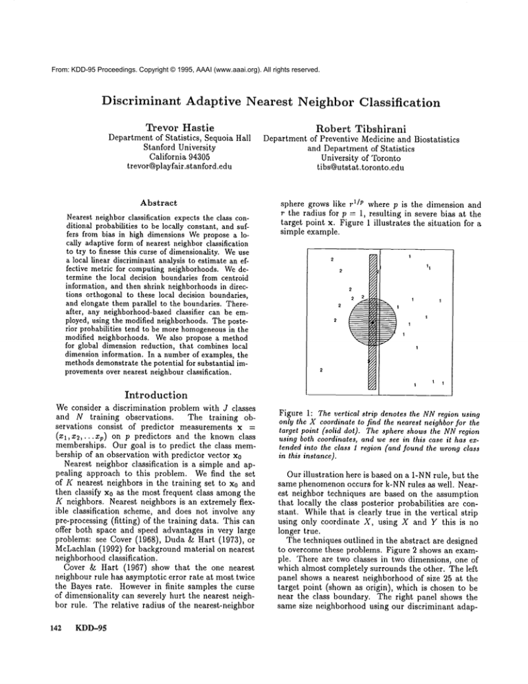
target point x. Figure 1 illustrates the situation for a
simple example.
Figure 1: The vertical strip denotes the NNregion using
only the X coordinate to find the nearest neighborfor the
target point (solid dot). The sphere shows the NNregion
using both coordinates, and we see in this case it has extended into the class 1 region (and found the wrongclass
in this instance).
Our illustration here is based on a 1-NNrule, but the
same phenomenonoccurs for k-NNrules as well. Nearest neighbor techniques are based on the assumption
that locally the class posterior probabilities are constant. While that is clearly true in the vertical strip
using only coordinate X, using X and Y this is no
longer true.
The techniques outlined in the abstract are designed
to overcome these problems. Figure 2 shows an example. There are two classes in two dimensions, one of
which almost completely surrounds the other. The left
panel shows a nearest neighborhood of size 25 at the
target point (shown as origin), which is chosen to
near the class boundary. The right panel shows the
same size neighborhood using our discriminant adap-
¯ components of distance in the null space of B* are
ignored;
¯ other components are weighted according to the
eigenvalues of B* when there are more than 2 classes
-- directions in which the centroids are more spread
out are weighted more than those in which they are
close
Thus this metric would result in neighborhoods similar to the narrow strip in figure 2: infinitely long in
the null space of B, and then deformed appropriately
in the centroid subspace according to how they are
placed. It is dangerous to allow neighborhoods to extend infinitely in any direction, so we need to limit this
stretching. Our proposal is
Figure 2: The leJt panel shows a spherical neighborhood
containing ~5 points. The right panel showsthe ellipsoidal
neighborhoodfound by the DANN
procedure, also containing ~5 points. Thelatter is elongatedalongthe true decision
boundary,and flattened orthogonalto it.
tive nearest neighbour procedure. Notice howthe modified neighborhoodextends further in the direction parallel to the decision boundary. As we will see in our
simulation studies, this new neighborhood can often
provide improvementin classification performance.
While the idea of local adaptation of the nearest
neighbour metric may seem obvious, we could find few
proposMsalong these lines in the literature.
A summary of previous work in given in section .
Discriminant adaptive
neighbors
nearest
Our proposal is motivated as follows. Consider first a
standard linear discriminant (LDA)classification procedure with K classes. Let B and W denote the between and within sum of squares matrices. In LDA
the data are first sphered with respect to W, then the
target point is classified to the class of the closest centroid (with a correction for the class prior membership
probabilities). Since only relative distances are relevant, any distances in the complementof the subspace
spanned by the sphered centroids can be ignored. This
complementcorresponds to the null space of B.
Wepropose to estimate B and Wlocally, and use
them to form a local metric that approximately behaves like the LDAmetric. One such candidate is
-1
= W-IBW
= W-1/2(W-
1/2BW-
1/2)W-I/2
-t/2.
= W-I/2B*W
+eI]W
* +el]W-1/~
= W-X/~[B
(2)
where e is some small tuning parameter to be determined. The metric shrinks the neighborhood in directions in which the local class centroids differ, with the
intention of ending up with a neighborhood in which
the class centroids coincide (and hence nearest neighbor classification is appropriate). With this goal in
mind one can think of iterating the procedure, and
thus successively shrinking in directions in which the
class centroids do not coincide.
Here is a summaryof the proposal.
Discriminant Adaptive Nearest Neighbor Classifier
O. Initialize the metric ~ = I, the identity matriz.
1. Spread out a nearest neighborhood of KMpoints
aroundthe test point x0, in the metric ~,,.
2. Calculate the weighted within and between sum of
squares matrices W and B using the points in the
neighborhood (see formula (8 below).
-~/2 +
3. Define a new metric ~,, = W-~/~[W-1/2BW
2eI]W-.
1[
4. Iterate steps 1, 2, and 3.
5. At completion, use the metric ~ for K-nearest neighbor classification at the test point x0.
The metric (2) can be given a more formal justification. Supposewe are classifying at a test point x0 and
find a single nearest neighbor X according to a metric
d(X, x0). Let p(j]x) be the true probability of class
at point x.
Weconsider the Chi-squared distance
(i)
whereB* is thebetween
sum-of-squares
in thesphered
space.Consider
theactionof ~ as a metricforcomputingdistances (x - x0)T~(x -- x0):
* it first spheres the space using W;
-x
= /2
W-~/2[W-V2BW-I/~
which measures the distance (appropriately weighted)
between the true and estimated posteriors.
Small
Hastie
143
r(X, x0) implies that the misclassification error rate
will be close to the asymptotic error rate for INN,
which is achieved when X = x0 or more generally when
p(jlX) = p(jlxo). Weshow that the first term in
metric (2) approximates r(X, x0).
Assuming that in the neighborhood xlj has a Gaussian distribution with mean pj and covariance E, we
obtain by a simple first order Taylor approximation
p(jIX) ~ p(jlx0) p( jlxo)(#j
- p) T~[~-l(x --
X0)
(4)
where # = ~j p(jlx0)pj.
Plugging this into (3) we
J
,’(X,x0)
~ Ep(jlx0) [(#j - #)TE-I(x 2 (5)
j=l
Thus the approximately best distance metric is
E-I ~j p(j[xo)(pj - p)(pj p) TE-I. Es timating E
by Wand ~j p(jlxo)(l~j
-#)(Pi by B giv esthe
first term in the metric (2).
By allowing prior uncertainty for the class meansPi,
that is, assumepj ,.~ N(v/, eI) in the sphered space,
obtain the second term in the metric (2).
Details
of the implementation
Define a weight function at x0 by
k(x, x0; h)
(6)
-- x0)ll).
Here E0 is an initial non-negative metric (often I), and
Ch is a symmetric real-valued function depending on a
parameter h. Weuse a lri-cube function defined over a
K-nearest neighborhood NK(x0) of x0. Formally,
define di = IIE1/2(xi -xo)ll, h maxiegK(xo)di and
define
(7)
k(xi,xo;h) = [1 (ddh)3]aI(Id<l
Let B(xo; Eo, h) and W(xo; Eo, h) be the weighted
between and within class sum of squares matrices,
where the weights assigned to the ith observation are
given by wi = k(xi, xo; Eo, h). That is,
J
U(0; r,0, h)
-
-
j=l
~j
--
Eyi=j
,oi
I Wi
(8)
EiN
to start with E0 = I (the identity matrix) and iterate
this procedure. The result is a metric E for use in
a nearest neighbor classification
rule at x0. In our
exampleswe try either a single step of this procedure,
or larger numberof iterations.
Some remarks
about
the DANN metric
It is natural to ask whether the mapping g(.) has
fixed point, and if it does, whether an iteration of the
form E ,-- g(E) converges to it. These questions seem
difficult to answer in general. To get some insight,
it is helpful to consider an equivalent form of the iteration. At each step we take a spherical neighborhood around the test point, estimate the metric I3, and
then transform the predictors via x"~’~ = El/2x °ta. At
completion we use a spherical nearest neighbor rule in
the final transformed space. It is easy to show that
this procedure is equivalent to the one given above. If
the metrics estimated in j iterations are El, E2, ¯ ¯ ¯ Ej,
then the effective metric for the original coordinates is
El12v,112
v,112~,~lZ~2
v.112"’’~j-l~j
v, ll2 vdl2"
j "-~j-1
"’’z"2
Expressed in this way, the fixed points of the itera-1 + eW-l = cI. In particular
tion satisfy W-1BW
a fixed point occurs when B is zero and W is proportional to the identity matrix, in the space of the
transformed coordinates.
In practice we find it moreeffective to estimate only
the diagonal elements of W, and assume that the off
diagonal elements are zero. This is especially true if
the dimension of the predictor space is large, as there
will be insufficient data locally to estimate the 2)
O(p
elements of W. With the diagonal approximation,
the two forms of the algorithm are not equivalent: we
use the version that transforms the space at each step
since a diagonal approximation makes most sense in
the transformed coordinates.
If the predictors are spatially or temporally related,
we might use a penalized estimate of Wthat downweights components of the covariance that correspond
to spatially noisy signals (Hastie, Buja & Tibshirani
1994). A related approach is to pre-filter the predictors
using a smooth basis, and then operate in the reduced
domain.
In the final neighborhood we perform K nearest
neighbor classification. An alternative approach would
be to use discriminant analysis to perform the classification, using the locally determined parameters. We
are currently investigating this approach.
Choice of tuning parameters
The DANN
procedure has a number of adjustable tunEN=I wi
ing
parameters:
(9)
KM: the number of nearest neighbors in the neighborhood
where 2j is the weighted mean of the Nj observations
NKM(x0) for estimation of the metric;
in the jth group. Finally, we let B(x0;E0, h) and
K : the numberof neighbors in the final nearest neighbor
B(x0; E0, h) determine the metric E in (2).
rule;
Notice that equations (8) and (2) produce a mapping
e : the "softening" parameter in the metric.
S0 -* E, say E = g(E0). An approach we explore
W(x0;
144
~0,
h)
KDD-95
E;=I
Eyi:j
Wi(Xi
--
:Xj)(XI
--
~j)T
Test set or cross validation could be used to estimate
an optimal values for these parameters. In the examples in the next section we instead use fixed choices.
The value of Kmmust be reasonably large since the
initial neighborhood is used to estimate a covariance:
we use KM= max(N/5, 50). To ensure consistency
one should take KMto be a vanishing fraction of N,
and should also use larger values for higher dimensional
problems. A smaller number of neighbors is preferable
for the final classification rule to avoid bias: we used
K = 5, and compared it to standard 5 nearest neighbors. Note that the metric (2) is invariant under nonsingular transformations of the predictors, and hence
it makessense to consider fixed values of e. After some
experimentation, we found that the value e = 1 works
well, and we use this value in the examples below.
where the B(i) are the local between sum of squares
matrices. This latter problem is solved by finding
the largest eigenvectors of the average between sum
of squares matrix ~1 B(i)/N.
LDAa~l Lo~l Subspac~-- K = 25
|1
1
I1
Dimension
Reduction
using
Local
Discriminant
Information
So far our technique has been entirely
"memory
based", in that we locally adapt a neighborhood about
a query point at the time of classification.
Here we
describe a method for performing a global dimension
reduction, by pooling the local dimension information
over all points in the training set. In a nutshell we consider subspaces corresponding to eigenvectors of the
average local between sum-of-squares matrices.
Consider first how linear discriminant analysis
(LDA)works. After sphering the data, it concentrates
in the space spanned by the class means~j or a reduced
rank space that lies close to these means. If ~ denote
the overall mean, this subspace is exactly the principal componenthyperplane for the data points ~j - ~,
weighted by the class proportions.
Our idea to compute the deviations :~j i locally in
a neighborhood around each of the N training points,
and then do an overall principal components analysis
for the N x J deviations. Here are the details. Let xi (i)
be the mean of class j vectors in a neighborhoodof the
ith training point, and ~(i) be the overall mean. All
means are weighted by the local class membershipproportions zr1 (i), j = 1,..., d. Let xi(i) = xj (i) the local centroid deviations. Weseek a subspace that
gets close in average weighted squared distance to all
N x J of these. Denoting by U (p x J) an orthonormal
basis for the k < p dimensional subspace,we minimize
the criterion
N
J
uuT)(0,
ass(u)
i=1 j=l
or the total weighted residual sum of squares. It is
not hard to show that minimizing RSS(U) amounts
to maximizing
tr
UT
B(i)
I1I
J
"
L
2222
2
I2 2
9
12//"
Figure 3: [Left Panel] Twodimensionalgaussian data with
two classes and correlation 0.65. The solid lines are the
LDAdecision boundaryand its equivalent subspacefor classification. The dashedlines wereproducedby the local procedure described in this section. [Right panel] Each line
segmentrepresents the local betweeninformation centered
at that point.
Figure 3 shows a simple illustrative
example. The
two classes are Gaussian with substantial within class
covariance between the two predictors Xl and X2. In
the left panel, the solid line is the Gaussian decision
boundary that optimally separates the classes. The
orthogonal vector labeled S is a one dimensional subspace onto which we can project the data and perform
classification.
Using the knowledgethat the data are
Gaussian, it is the leading discriminant direction. The
broken lines are the boundaries and equivalent subspace produced by our procedure. In the right panel,
each line segment represents the local between information centered at that point. Our procedure uses a
principal componentsanalysis of these N x J line segments to produce the broken line subspace in the left
panel.
To allow combination of the local between information in a meaningful way, notice that we have not
sphered the data locally before computing the mean
deviations. A justification for this is that any local
spherical windowcontaining two classes, say, will have
approximately a linear decision boundary orthogonal
to the vector joining the two means.
Figure 4 shows the eigenvalues of the average between matrix for an instance of a two class, 4 dimensional sphere model with 6 noise dimensions. The decision boundary is a 4 dimensional sphere, although
locally linear (full details of this exampleare given in
the next section). For this demonstration we randomly
rotated the 10 dimensional data, so that the dimensions to be trimmed are not coordinate directions. The
eigenvalues show a distinct change after 4 (the correct
Hastie
145
For all methods, the predictors were first standardized so as to have zero meanand unit variance over the
training set, and the test set predictors was standardized by the corresponding training mean and variance.
The training and test set sizes were 200 and 500, unless
indicated otherwise.
4D Spherewith 6 noise Variables
d
2
4
6
8
10
Order
Figure 4: The eigenvalues of the average between matrix
for the 4Dsphere -I- 6 noise variable problem.Usingthese
first four dimensions followed by our DANN
nearest neighbor routine, we get better performancethan 5NNin the real
4Dsubspaee.
dimension), and using our DANN
classifier in these
four dimensions actually beats ordinary 5NNin the
known four dimensional sphere subspace.
It is desirable to automate the dimension reduction
operation. Since our local information is based on
spherical neighborhoods (potentially in high dimensions), we find an iterative approach most successful. Weapply this procedure in the full space, and
use cross-validated DANN
to find the best nested subspace (with a built in bias towards larger subspaces).
Wethen successively repeat these operations in the
new subspaces, until no further reduction is deemed
suitable by CV. Using DANN
in this final subspace is
what we have labelled sub-DANNin the boxplots of
figures 5.
Examples
The methods
In the following examples we compareseveral classification approaches:
¯ LDA--linear discriminant analysis
¯ reduced LDA--linear discriminant restricted to the
(known) relevant subspace, where appropriate.
¯ 5-NN: 5 nearest neighbor classification
¯ reduced 5-NN
¯ DANN--Discriminant adaptive nearest neighbor,
one iteration.
¯ iter-DANN-- Discriminant adaptive nearest neighbor, five iterations.
¯ sub-DANN--Discriminant adaptive nearest neighbor, with automatic subspace reduction. This is described in section .
146
KDD-95
The problems
1. 2 Dimensional Gaussian with 1.~ Noise.Two Gaussian classes in two dimensions (X1,X2) separated
by 2 units in X1. The predictors have variance (1,2)
and correlation 0.75. The additional 14 predictors
are independent standard Gaussians.
2. Unstructured with 8 Noise. There are 4 classes each
with 3 spherical bivariate normal subclasses, having standard deviation 0.25. The means of the 12
subclasses were chosen at random (without replacement) from the integers [1, 2,... 5] x [1, 2,...5]. Each
training sample had 20 observations per subclass, for
a total of 240 observations. The additional 8 predictors are independent standard Gaussians.
3. 4 Dimensional Spheres with 6 Noise. In this example there are 10 predictors and 2 classes. The last 6
predictors are noise variables, with standard Gaussian distributions, independent of each other and the
class membership.The first four predictors in class
1 are independent standard normal, conditioned on
the radius being greater than 3, while the first four
predictors in class 2 are independent standard normal without the restriction. The first class almost
completely surrounds the second class in the four dimensional subspace of the first four predictors. This
example was designed to see if DANN
could improve
upon nearest neighbors in the presence of noise variables.
4. 10 Dimensional Spheres. As in the previous example there are 10 predictors and 2 classes. Nowall 10
predictors in class 1 are independent standard normal, conditioned on the radius being greater than
22.4 and less than 40, while the predictors in class
2 are independent standard normal without the restriction. In this example there are no pure noise
variables, the kind that a nearest neighbor subset
selection rule might be able weed out. At any given
point in the feature space, the class discrimination
occurs along only one direction. Howeverthis direction changes as we moveacross the feature space and
all variables are important somewherein the space.
The first class almost completely surrounds the second class in the full ten-dimensional space.
Discussion of results
The results for the simulated examples are summarized
in Figures 5.
DANN
seems to do as well as 5-NNacross the board,
and offers significant improvements in problems with
noise variables. DANN
does not do as well as reduced
TwoGausslanewith Noise
Unstructuredwith Noise
Enorrel¢l fCalJve
Io ,,~-~1
I
,,
I
T
I
,...............
i............
....f-I_;
............
.
i
!
1
)fii
!
770
l
4-D Spherein 10-D
¯
T
o
"i
E/TOt r~ r~ll to LDA
°
[
-
lI
|
¯¯
=
°
I
,
T
T
I
I
l
-’
I
--
I
I
l
+* ~¢ i
10-D sphere in 10-D
*
l
I
i
1
l
i
1
!
Figure 6: Relative error rates ol the methodsacross the
8 simulated problems. In the top panel the error rate has
been divided by the error rate 5-NN,on a simulation by
simulation basis. In the bottom panel we have divided by
the error rate ol LDA.
E3
1
1
.
,’itii
o
.+- ,,,+ <>¢//
Spectral band 1
Speclml band 2
Spectral
band 3
Figure5: Boxplotsof error rates over ~0 simulations.
nearest neighbors in problems1 and 3: this is not surprising since in effect we are giving the nearest neighbor rule the information that DANN
is trying to infer
from the training data. A nearest neighbor method
with variable selection mightdo well in these problems:
howeverthis procedurecan be foiled by by rotating the
relevant subspace awayfrom the coordinate directions.
On the average there seems to be no advantage in
carrying out morethan one iteration of the DANN
procedure. The subspace DANNprocedure is the overall winner, producingbig gains in problemsadmitting
global dimensionreduction.
The top panel of Figure 6 shows error rates relative
to 5-NN, accumulatedacross 8 x 20 simulated problems
(these 4 and another 4 described in Hastie & Tibshirani
(1995). The bottom panel shows the rates relative
Spectral band 4
Land use (Actual)
Land use (Predicted)
Figure 7: The first four imagesare the satellite images
in the four spectral bands. The fifth imageis the known
classification, andthe final imageis the classification map
producedby linear discrlmlnantanalysis.
LDA.
Wesee that DANNis 20-30% better than 5-NN on
the average, and is at most 20%worse. DANN
is also
better than LDAon the average but can be three times
worse (in problem2).
Image Classification
Example
Imagescene classification is an importantand difficult
problem. The example we consider here is classifying
satellite images of an area of the earth’s surface into
land and vegetation type. Other examplesinclude classification of X-rays, such as mammograms,
into normal
or calcified into normalor cancerousregions.
Figure 7 shows four spectral bands of a section of
land, two in the visible spectrum (red and green)
N
N
N
N
X
N
N
N
N
A Pixel and its
8 neighbors
Figure8: Thepixel intensities of the 8-neighborsof a pixel
(anditself) are usedas featuresfor classification
Hastie
147
and two in the infra red spectrum. These data are
taken from the STATLOG
projects archive (Michie,
Spigelhalter & Taylor 1994)1. The goal is to classify each pixel into one of 7 land types: red soil,
cotton, vegetalion stubble, mixture, grey soil, damp
grey soil, very damp grey soil. Weextract for each
pixel its 8-neighbors, as depicted in figure 8, giving us
(8+ 1)x 4 = 36 features (the pixel intensities) per pixel
to be classified. The data come scrambled, with 4435
training pixels and 2000 test pixels, each with their
36 features and the knownclassification. Included in
figure 7 is the true classification, as well as that produced by linear discriminant analysis. Figure 9 shows
SatelliteImage
Classification
..h o
o
0°.
o
5
10
15
20
25
~rnee,s~n
STATLOG
results
LDA
Figure 10: Miscla.ssification results as a function of subspace size, for the satellite imagedata
ogistic
SMART
QDA
NewlDC4.5
CART
ALLOCSO
Nueral
RBF
LVQ
K-NN
8
<5
)AN
i
i
i
i
i
t
i
2
4
6
8
10
12
14
Method
Figure 9: Misclassification results of a variety of classification procedures on the satellite imagetest data (taken
from Michieet al. (1994)).
the results reported in Michie et al. (1994) for a variety of classifiers; they reported the best result for
5-NNclassification. Included in the figure is the result
for DANN,which has outperformed 5-NN. Wealso ran
the subspace version of DANN,
and figure 10 shows the
sequence of of test-error results as a function of subspace size. Again, a low-dimensional subspace actually
improves the misclassification error.
Discussion
Wehave developed an adaptive form of nearest neighbor classification that can offer substantial improvements over standard nearest neighbors method in some
problems. Wehave also proposed a method that uses
local discrimination information to estimate a subspace
for global dimension reduction.
Short & Fukanaga (1980) proposed a technique close
to ours for the two class problem. In our terminology
they used our metric with W = I and e = 0, with B
1The authors thank C. Taylor and D. Spiegelhalter for
makingthese images and data available
148
KDD-95
determined locally in a neighborhood of size KM. In
effect this extends the neighborhood infinitely in the
null space of the local between class directions, but
they restrict this neighborhood to the original KM observations. This amounts to projecting the local data
onto the line joining the two local centroids. In our
experiments this approach tended to perform on average 10%worse than our metric, and we did not pursue
it further. Short & Fukanaga (1981) extended this
J > 2 classes, but here their approach differs even
more from ours. They computed a weighted average
of the J local centroids from the overall average, and
project the data onto it, a one dimensional projection.
Even with e = 0 we project the data onto the subspace containing the local centroids, and deform the
metric appropriately in that subspace. Myles & Hand
(1990) recognized a shortfall of the Short and Fukanaga
approach, since the averaging can cause cancellation,
and proposed other metrics to avoid this. Although
their metrics differ from ours, the Chi-squared motivation for our metric (3) was inspired by the metrics
developed in their paper. Wehave not tested out their
proposals, but they report results of experiments with
far more modest improvements over standard nearest
neighbors than we achieved.
Friedman (1994) proposes a numberof techniques for
flexible metric nearest neighbor classification. These
techniques use a recursive partitioning style strategy
to adaptively shrink and shape rectangular neighborhoods around the test point. Friedman also uses derived variables in the process, including discriminant
variates. With the latter variables, his procedures have
some similarity to the discriminant adaptive nearest
neighbor approach.
Other recent work that is somewhatrelated to this
is that of Lowe(1993). He estimates the covariance
matrix in a variable kernel classifier using a neural network approach.
There are a number of ways in which this work might
be generalized. In some discrimination problems, it
is natural to use specialized distance measures that
capture invariances in the feature space. For example Simard, LeCun & Denker (1993), IIastie, Simard
& Sackinger (1993), use a transformation-invariant
metric to measure distance between digitized images
of handwritten numerals in a nearest neighbor rule.
The invariances include local transformations of images such as rotation, shear and stroke-thickness. An
invariant distance measure might be used in a linear
discriminant analysis and hence in the DANNprocedare.
Another interesting possibility wouldbe to apply the
techniques of this paper to regression problems. In this
case the response variable is quantitative rather than
a class label. Natural analogues of the local between
and within matrices exist, and can be used to shape
the neighborhoods for near-neighbor and local polynomial regression techniques. Likewise, the dimension
reduction ideas of section can also be applied. There
is a strong connection betweenthe latter and the Sliced
Inverse Regression technique of Duan & Li (1991) forsubspace identification.
Weare currently exploring
these directions.
Acknowledgments We thank Jerome Friedman for
sharing his recent work, which stimulated us to embark
on this project, and for manyenjoyable conversations.
The second author was supported by a grant from
the Natural Sciences and Engineering Research Council of Canada.
Lowe, D. G. (1993), Similarity metric learning for
variable kernel classifier, Technical report, Dept. of
CompSci, Univ. of British Columbia.
McLachlan, G. J. (1992), Discriminant Analysis and
Statistical Pattern Recognition, Wiley, NewYork.
Michie, D., Spigelhalter, D. & Taylor, C., eds (1994),
Machine Learning, Neural and Statistical Classification, Ellis IIorwoodseries in Artificial Intelligence,
Ellis Horwood.
Myles, J. &Hand, D. J. (1990), ’The multi-class metric
problem in nearest neighbour discrimination rules’,
Pattern Recognition 23, 1291-1297.
Short, 1~. &Fukanaga, K. (1980), A new nearest neighbor distance measure, in ’Proc. 5th IEEE Int. Conf.
on Pattern Recognition’, pp. 81-86.
Short, R. & Fukanaga, K. (1981), ’The optimal
distance measure for nearest neighbor classification’, IEEE transactions of Information Theory IT27, 622-627.
Simard, P. Y., LeCun,Y. & Denker, J. (1993), Efficient
pattern recognition using a new transformation distance, in ’Advances in Neural Information Processing
Systems’, Morgan Kaufman, San Mateo, CA, pp. 5058.
References
Cover, T. (1968), Rates of convergence for nearest
neighbor procedures, in ’Proc. Hawaii Inter. Conf.
on Systems Sciences’, Western Periodicals, Honolulu,
pp. 413-415.
Cover, T. & Hart, P. (1967), ’Nearest neighbor pattern classification’,
Proc. IEEE Trans. Inform. Theory pp. 21-27.
Duan,N. & Li, K.-C. (1991), ’Slicing regression: a linkfree regression method’, Annals of Statistics pp. 505530.
Duda, R. O. &IIart, P. E. (1973), Pattern classification and scene analysis, Wiley, NewYork.
Friedman, J. (1994), Flexible metric nearest neighbour
classification, Technical report, Stanford University.
IIastie, T. &Tibshirani, R. (1995), Discriminant adaptive nearest neighbor classification, Technical report,
Stanford University Statistics Department.
IIastie, T., Buja, A. &Tibshirani, R. (1994), Penalized
discriminant analysis, To appear, Annals of Statistics.
IIastie, T., Simard, P. &Sackinger, E. (1993), Learning prototype models for tangent distance, Technical
report, AT&Bell Labs.
Hastie
149