From: KDD-97 Proceedings. Copyright © 1997, AAAI (www.aaai.org). All rights reserved.
Fast Committee Machines for Regression and Classification
Harris Drucker
Monmouth University
West Long Branch, NJ 07764
drucker@monmouth.edu
Abstract
In many data mining applications we are given
a set of training examples and asked to
construct a regression machine or a classifier
that has low prediction error or low error rate
on new examples, respectively. An important
issue is speed especially when there are large
amounts of data. We show how both
classification and prediction error can be
reduced by using boosting techniques to
implement committee machines. In our
implementation of committees using either
classification trees or regression trees, we show
how we can trade off speed against either error
rate or prediction error.
combining regressors using boosting techniques. In
boosting each machine is trained on different subsets of
the training set. The first machine is trained on
examples picked with replacement from the original
training set. We then pass all the training patterns
through this first machine and note which ones are in
error (in classification). For regression machines, those
patterns whose predicted values differ most from their
observed values are defined to be “most” in error. For
those patterns in error, the sampling probabilities are
adjusted so that difficult examples are more likely to be
picked as members of the training set for the second
machine. Thus, different machines are better in different
parts of the observation space. Regressors are combined
using the weighted median while classification machines
are combined using a weighted sum of the hypotheses.
Details of these weighting scheme are discussed later.
Introduction
Boosting techniques [Trucker (1993, 1994, 1996a),
Freund and Schapire (1996a,b), Schapire (lQQO)]allows
one to obtain smaller prediction errors (in regression)
and lower error rates (in classification) using multiple
predictors. The ensemble of classifiers is often called a
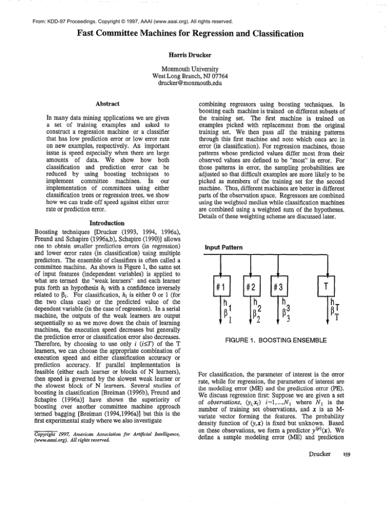
committee machine. As shown in Figure 1, the same set
of input features (independent variables) is applied to
what are termed the “weak learners” and each learner
puts forth an hypothesis hi with a confidence inversely
related to pi. For classification, hi is either 0 or 1 (for
the two class case) or the predicted value of the
dependent variable (in the case of regression). In a serial
machine, the outputs of the weak learners are output
sequentially so as we move down the chain of learning
machines, the execution speed decreases but generally
the prediction error or classification error also decreases.
Therefore, by choosing to use only i (ST) of the T
learners, we can choose the appropriate combination of
execution speed and either classification accuracy or
prediction accuracy. If parallel implementation is
feasible (either each learner or blocks of N learners),
then speed is governed by the slowest weak learner or
the slowest block of N learners. Several studies of
boosting in classification [Breiman (1996b), Freund and
Schapire (1996a)] have shown the superiority of
boosting over another committee machine approach
termed bagging [Breiman (1994,1996a)] but this is the
first experimental study where we also investigate
Copyright 1997, American Association for ArtzjTcial Intelligence,
(nww.aaai.org). All rights reserved.
input Pattern
m
w
#I
w2
hl
P
11
h
2
P
72
FIGURE 1. BOOSTING ENSEMBLE
For classification, the parameter of interest is the error
rate, while for regression, the parameters of interest are
the modeling error (ME) and the prediction error (PE).
We discuss regression first: Suppose we are given a set
of observations, (vi,Xi) i=l,...,N1 where Ni is the
number of training set observations, and x is an Mvariate vector forming the features. The probability
density function of (y,x) is fixed but unknown. Based
on these observations, we form a predictor y@)(x). We
define a sample modeling error (ME) and prediction
Drucker
159
error (PE):
functional form as long as LE [O,l]. If we let
ME =
$yi”-yp)(xj)]2
N2 i=l
where yfp)&) is the prediction for the i’th test example,
yi is the i’th observation, and y:) is the “truth”. The
parameters of y@)(x) are obtained from the Nr training
set observations but the yi and xi in the above
summations are obtained from a set of N2 observations
(the test set) never seen before. If the noise is additive,
then Yi=Yf)+ni where ni is the i’th sample of the noise.
Furthermore, if E[n] = 0 and E[~inj]=Gij02, then we
may take the expectation with respect to (y,X) and
obtain (Breiman and Spector, 1992):
D=sup 1yp)&)
then we have
examined:
i
Boosting Algorithm
The theory behind the boosting algorithms are presented
elsewhere(Freund and Schapire, 1996b). Here we
present the boosting algorithm for regression:
Repeat the following while the average loss z defined
below is less than .5 .
1. The probability that training sample i is in the
training set is pi=WiaWi where the summation is over
all members of the training set. Initially, the wi are set
equal to unity. Pick Ni samples (with replacement) to
form the training set. This may be implemented by
marking a line of length xwwi and subsections of length
wi . A uniform number picked from the range [O,cWi]
and landing in section i corresponds to picking pattern i.
2. Construct a regression machine t from that training
set. Each machine makes a hypothesis: h,:x+y
3. Pass every member of the training set through this
machine to obtain a prediction yp)(xJ i=l, ..,N 1.
160
KDD-97
loss functions
-Yi I
i
D2
-
Li=l - exp
12
I yfp’(Xi>
-yi I
D
[
we
(linear)
D
L = 1 Yfp’b?) - Yi
(square law)
1
(exponential)
5. Calculate an average loss: iZ=?Lj*i
i=l
E[PE] = 02+E[ME]
This shows us that even if we know the model exactly,
there is a minimum prediction error due to the noise. Our
problem will be that the modeling error is also nonzero
because we have to determine the model in the presence
Since we don’t know the probability
of noise.
distributions, we approximate the expectation of the ME
and PE using the sample ME (if the truth is known) and
sample PE and then average’over multiple experiments.
Similarly, for the classification case, we have a training
error for those examples we train on and a test error for
the test examples tested on a machine constructed using
the training examples. Our implementation of each
weak learner is a tree, either a regression tree or a
classification
of their ease of
tree because
implementation, small training time, and fast execution
speed.
three candidate
1Y%i)
L=
-yi 1 i=l,...,Nr
-
6. Form j3=-&.
predictor. Low
prediction.
p is a measure of confidence in the
p
means high confidence
in the
7. Update the weights: wi-+w$**[l-Lj],
where **
indicates exponentiation. The smaller the loss, the more
the weight is reduced making the probability smaller
that this pattern will be picked as a member of the
training set for the next machine in the ensemble.
8. For a particular input xi, each of the T machines
makes a prediction h,, t=l,...,T. Obtain the cumulative
prediction hf using the T predictors:
hf= inf
This is the weighted median. Intuitively, the effect of
varying the weight wi to give more emphasis to
“difficult” examples means that each subsequent
machine has a disproportionately harder set of examples.
Thus, the average loss tends to increase as we iteLate
through the algorithm and ultimately the bound on L is
not satisfied and the algorithm terminates,
For classification, we replace steps 4 and 8 above. In
step 4, the loss for pattern i becomes Liz I h,(i) - c(i) 1
where h,(i) is the hypothesis of machine t (0 or 1) and
c(i) is the correct classification (either 0 or 1). The issue
of multiclass classification will be discussed in the
conclusion. In step 8, the final hypothesis is:
T
I;(bgl)
‘=I
Pt
T
h,(i)2L~10gL
2 t=1
otherwise
Pt
Note that the examples referred to in the algorithm above
only refers to training examples and we usually observe
convergence to zero classification error or zero
prediction error on these training examples. However,
we are interested in the performance on a test set.
Therefore, at each stage of boosting, we pass the test set
through the ensemble and use step 8 to obtain the test
performance. How well we generalize to the test set will
depend on our choice of weak learner, e.g., neural net,
tree, nearest neighbor classifier.
Trees
Regression trees are based on Breiman’s CART
[Breiman, 19941. In this implementation of regression
trees, one starts (at the top) with a main node that
examines a specified feature of the input pattern and
compares its value to a “separator” value assigned to
that node. If the value of the feature is less than or equal
to the separator, we continue down the left side of the
tree, else the right side. Each of the children of the main
node has a specified feature and separator value for that
feature. Each parent node has two children nodes and
those children nodes become parents of their children.
Depending on the values of the features for the input
pattern, we continue down the tree, at each node going
left or right until we reach a terminal leaf. At the
terminal leaves, we assign a hypothesis that is the
predicted value of the regression, For classification trees,
the building criterion is based on an information
theoretic basis found in C4.5 [Quinlan, 19931. To
generalize well to as an yet unseen test set, we then
prune back the trees using a separate pruning set.
Pruning Mingers, 19891 performs two essential tasks (a)
it increases the execution speed because the tree is
smaller and (b) the generalization is better.
Experiments
We tried several cases of classification and regression
using the techniques described above. The first
regression problem was based on that of Friedman
(1991), which is a nonlinear prediction problem which
has 10 independent variables that are uniform in [O,l]
Here we can determine both the modeling and prediction
error.
where n is normal (0,l). Therefore, only five predictor
variables are really needed, but the predictor is faced
with the problem of trying to distinguish the variables
that have no prediction ability ( x6 to xl0 ) from those
that have predictive ability ( x1 to x5 ). For different
training set sizes (pruning size is 20% of the training set
size) and a test set of of size 10,000 we plot (Figure 2)
execution speed (on a SparcStation 20) versus the
prediction error on the test set. Each data point is the
average of ten samples. Generally as we increase the
number of trees in the ensemble (thereby decreasing the
execution speed), the prediction error decreases. Because
of the inherent noise floor in this prediction problem, the
PE tends to asymptote with increasing number of trees
and large enough number of examples. There is a
continuum of prediction error versus speed trade-offs,
We can show similar behavior on other regression and
classification problems.
Discussion
and Conclusions
Discussion and Conclusions” We have shown how to
use boosting to reduce error rates in classification and
prediction error in regression using classification trees
and regression trees, respectively. Of critical importance
is the pruning of the trees by using a separate set of
pruning data after the tree has been initially grown using
the training set. Pruning both increases the speed and
improves the generalization to samples as yet unseen.
By picking the appropriate number of trees in the
ensemble, one can trade off speed versus performance.
If the speed performance is not acceptable (but the error
rate or prediction error is), then one choice is a parallel
architecture. Generally, there are between forty and
seventy trees in an ensemble and therefore the speed
would increase by those factors (but only approximately
since not all trees are the same size). If error rate or
prediction error is the issue, then another possibility is to
build a single neural network. Generally a single neural
network is slower than these ensembles because trees
just implement simple IF statements, while neural
networks need to implement both multiplication and
some sigmoid function as the transfer functions.
However, these issues must be decided on a case-by-case
basis.
Acknowledgements
Part of this work was performed under ARPA contract
NOOO14-94-C-0186while at Lucent Technologies.
References
Breiman, L. (1996),“Bias, Variance, and Arcing
Classifiers Technical Report 460, Department of
Statistics, University of California, Berkeley, CA.
Annals of Statistics (to be published)
Breiman, L. and Spector, P., (1992). “Submodel
Selection and Evaluation in Regression. The X-Random
Case”, International Statistical Review, 60, 3, pp.291319.
Breiman, L., Friedman, H.H., Olshen, R.A. and Stone,
C.J. (1984), Classfication and Regression Trees,
Wadsworth International Group.
Breiman, L. (1996) “Bagging Predictors” Machine
Learning, vol. 26, No. 2,pp. 123-140.
Breiman, L. (1996),“Bias, Variance, and Arcing
Classifiers Technical Report 460, Department of
Statistics, University of California, Berkeley, CA.
Annals of Statistics (to be published)
Drucker, H., (1997), “Improving Regressors using
Boosting Techniques”, 1997 International Conference on
Machine Learning.
Drucker
161
7
6
C-+
/
/
5
E;FiIjctlon
200
Samples
/
r-
I
4
Speed
Figure
2.
In
PredictIon
regressions
error
v-rsus
second
for
a regression
problem
Drucker, H., Schapire, R.E., Simard, P., (1993),
“Boosting Performance in Neural Networks”,
International Journal of Pattern Recognition and
Artificial Intelligence, 7,4, pp. 705719.
“Experiments with a New Boosting Algorithm”,
Machine Learning: Proceedings of the Thirteenth
Conference, ed: L. Saitta, Morgan Kaufmann, pp.
148-156.
Drucker, H., Cortes, C., Jackel, LD., LeCun, Y.,
Vapnik V., (1994). “Boosting and Other
Ensemble Methods”, Neural Computation , 6, 6,
pp. 1287-1299. pp. 1287-1299.
Freund, Y. and Schapire, R.E. (1996b) “A
decision-theoretic
generalization
of on-line
learning and an application to boosting”, at web
site:
http://www.research.att.com~yoav.
or
http://www.research.att.com/orgs/ssr/people/”yoav.
An extended abstract appears in the Proceedings
of the Second European
Conference
on
Computational Learning Theory, Barcelona,
Springer-Verlag, March, 1995, pp. 23-37.
Drucker, H., (1996), “Fast Decision Tree
Ensembles for Optical Character Recognition”,
Proceedings of the Fiflh Annual Symposium on
Document Analysis and Information Retrieval
Drucker, H., (1996) and Cortes, C., “Boosting
Decision Trees”, Neural Information Processing
8, ed: D.S. Touretzky, M,C. Mozer and M.E.
Hasselmo. Morgan Kaufmann, pp.479-485.
Drucker, H., (1997), “Improving Regressors using
Boosting Techniques”, submitted to the 1997
conference on Machine Learning.
Freund, Y., (1990), “Boosting a Weak Learning
Algorithm by Majority”, Proceedings of the Third
Workshop on Computational Learning Theory,
Morgan-Kaufmann, 202-216
Freund,
162
per
speed
KDD-97
Y.
and
Schapire,
R.E.
(1996a)
Friedman J., (1991), “Multivariate Adaptive
Regression Splines”, Annul of Statistics, vol 19,
No. 1, pp. l-141
J. Mingers (1989a), “An Empirical Comparison of
Pruning Methods for Decision Tree Induction”,
Machine Learning, 4~227-243.
J.R.Quinlan (1993), C4.5:
Programs
Machine Learning, Morgan Kauffman.
For
Schapire, R.E., (1990), “The Strength of Weak
Learnability”, Machine Learning, 5, 2, pp. 197227.