Improving the Separability of a Reservoir Facilitates Learning Transfer
David Norton and Dan Ventura
Computer Science Department
Brigham Young University
ghotikun@hotmail.com, ventura@cs.byu.edu
Abstract
We use a type of reservoir computing called the liquid
state machine (LSM) to explore learning transfer. The
Liquid State Machine (LSM) is a neural network model
that uses a reservoir of recurrent spiking neurons as a
filter for a readout function. We develop a method of
training the reservoir, or liquid, that is not driven by
residual error. Instead, the liquid is evaluated based
on its ability to separate different classes of input into
different spatial patterns of neural activity. Using this
method, we train liquids on two qualitatively different
types of artificial problems. Resulting liquids are shown
to substantially improve performance on either problem
regardless of which problem was used to train the liquid, thus demonstrating a significant level of learning
transfer.
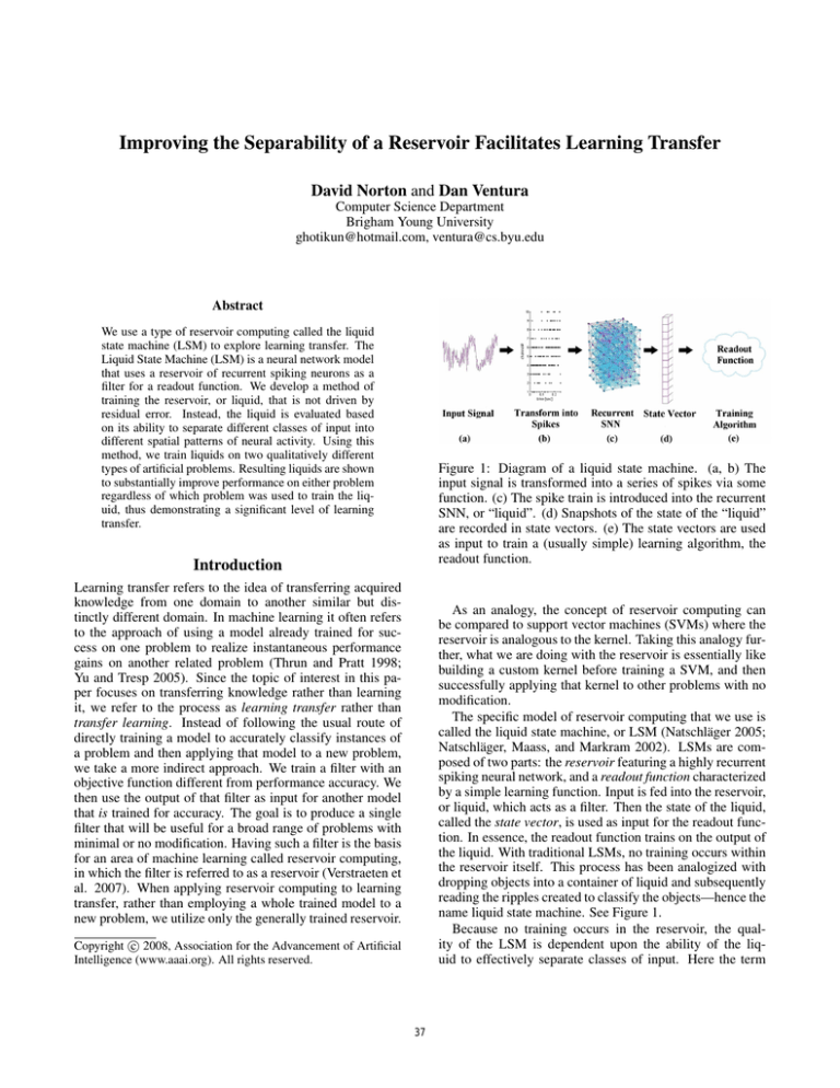
Figure 1: Diagram of a liquid state machine. (a, b) The
input signal is transformed into a series of spikes via some
function. (c) The spike train is introduced into the recurrent
SNN, or “liquid”. (d) Snapshots of the state of the “liquid”
are recorded in state vectors. (e) The state vectors are used
as input to train a (usually simple) learning algorithm, the
readout function.
Introduction
Learning transfer refers to the idea of transferring acquired
knowledge from one domain to another similar but distinctly different domain. In machine learning it often refers
to the approach of using a model already trained for success on one problem to realize instantaneous performance
gains on another related problem (Thrun and Pratt 1998;
Yu and Tresp 2005). Since the topic of interest in this paper focuses on transferring knowledge rather than learning
it, we refer to the process as learning transfer rather than
transfer learning. Instead of following the usual route of
directly training a model to accurately classify instances of
a problem and then applying that model to a new problem,
we take a more indirect approach. We train a filter with an
objective function different from performance accuracy. We
then use the output of that filter as input for another model
that is trained for accuracy. The goal is to produce a single
filter that will be useful for a broad range of problems with
minimal or no modification. Having such a filter is the basis
for an area of machine learning called reservoir computing,
in which the filter is referred to as a reservoir (Verstraeten et
al. 2007). When applying reservoir computing to learning
transfer, rather than employing a whole trained model to a
new problem, we utilize only the generally trained reservoir.
As an analogy, the concept of reservoir computing can
be compared to support vector machines (SVMs) where the
reservoir is analogous to the kernel. Taking this analogy further, what we are doing with the reservoir is essentially like
building a custom kernel before training a SVM, and then
successfully applying that kernel to other problems with no
modification.
The specific model of reservoir computing that we use is
called the liquid state machine, or LSM (Natschläger 2005;
Natschläger, Maass, and Markram 2002). LSMs are composed of two parts: the reservoir featuring a highly recurrent
spiking neural network, and a readout function characterized
by a simple learning function. Input is fed into the reservoir,
or liquid, which acts as a filter. Then the state of the liquid,
called the state vector, is used as input for the readout function. In essence, the readout function trains on the output of
the liquid. With traditional LSMs, no training occurs within
the reservoir itself. This process has been analogized with
dropping objects into a container of liquid and subsequently
reading the ripples created to classify the objects—hence the
name liquid state machine. See Figure 1.
Because no training occurs in the reservoir, the quality of the LSM is dependent upon the ability of the liquid to effectively separate classes of input. Here the term
c 2008, Association for the Advancement of Artificial
Copyright Intelligence (www.aaai.org). All rights reserved.
37
Separation is divided into two parts, the inter-class distance, Cd (t), and the intra-class variance, Cv (t). Cd (t) is
defined by Equation 1 and is the mean distance between the
center of mass for every pair of classes. The center of mass
for each class, µ(Om (t)), is calculated with Equation 2. For
clarity, we use | · | notation for set cardinality, and k·kk notation for the Lk -norm.
“effectively separate” is defined as the ability of a liquid
to yield unique state vectors for different classes of input,
which will allow the readout function to attain acceptable
accuracy. Typically, the liquid is created randomly according to some carefully selected parameters specific to
the problem at hand. This parameter selection has been
the topic of much research (Goodman and Ventura 2005;
Verstraeten et al. 2007) although the research has not yet
led to a consistent and general method of generating liquids
for all problems (Verstraeten, Schrauwen, and Stroobandt
2007). Even when adequate parameters for a given problem
have been implemented, the creation of a useful liquid is not
guaranteed. Typically hundreds or even thousands of liquids
will be created to find a suitable filter. Fortunately, once such
a liquid is discovered, the results of the LSM are comparable with the state-of-the-art (Goodman and Ventura 2006;
Verstraeten et al. 2007; 2005). Also, once a suitable liquid
is found, it can typically be presented with other problems
to good effect—the essence of learning transfer.
Since traditionally the liquids are randomly generated, the
process of creating an effective liquid has not incorporated
learning. However, we have developed a method for creating effective liquids in an LSM without having to rely on the
generation of many random liquids. We do so by randomly
creating a liquid in the traditional fashion and then adjusting
the liquid’s architecture until it can “effectively separate” as
defined above. We present the liquid with sample data, observe the resulting behavior, and then use these observations
to make the necessary changes to the liquid. Although this
approach uses training data to modify the liquid, the objective function is based on separation rather than error. The
goal is to create a liquid that will effectively separate classes
of input into different patterns of state vectors. Afterwards,
the readout function will learn to extract information from
the state vectors via traditional error-driven learning.
In this paper we show that using this indirect approach to
training a recurrent spiking neural network facilitates learning transfer. We will begin by defining a metric, called separation, that will be used to evaluate the quality of a liquid. Next we will outline our method of creating effective liquids, called Separation Driven Synaptic Modification
(SDSM). Then we will describe two artificial problems we
use to evaluate our algorithms. Finally we will show the results of our experiments and draw conclusions. All of the
LSMs used in this paper are created using CSIM, “a tool for
simulating heterogeneous networks composed of different
model neurons and synapses” (Natschläger 2005).
Cd (t) =
N X
N
X
kµ(Om (t)) − µ(On (t))k2
N2
m=1 n=1
P
µ(Om (t)) =
on ∈Om (t)
on
|Om (t)|
(1)
(2)
Cv (t) is defined by Equation 3 and is the mean variance of
every cluster, or class, of state vectors. ρ(Om (t)) is the average amount of variance for each state vector within class m
from the center of mass for that class. It is shown in Equation 4.
Cv (t) =
N
1 X
ρ(Om (t))
N m=1
P
ρ(Om (t)) =
on ∈Om (t)
kµ(Om (t)) − on k2
|Om (t)|
(3)
(4)
Separation can now be defined by Equation 5. Cv (t) is incremented by one to ensure that separation never approaches
∞.
Cd (t)
(5)
Cv (t) + 1
Here Ψ is the liquid that produced the set of state vectors,
O(t). Separation essentially measures the mean distance
between classes of state vectors divided by the average variance found within those classes.
In Figure 2 we show that separation does correlate with
the effectiveness of a liquid. Here, effectiveness is measured
as the accuracy of the LSM at classifying inputs in an artificial problem. One thousand liquids were generated with
varying parameter settings to create a large variety of separation values. The artificial problem consisted of five input
classes expressed as spiking patterns for four input neurons.
Separation was calculated with only three examples from
each class. Since we were not applying a synapse modifying
algorithm to the liquids, only one iteration, t, was observed.
The correlation coefficient between accuracy and separation
is a convincing 0.6876.
SepΨ (O(t)) =
Separation
Separation is a metric used to determine the effectiveness of
a liquid. It essentially measures how well the liquid separates different classes of input into different reservoir states,
or state vectors, and is analogous to supervised clustering.
Separation is calculated by dividing a set of state vectors,
O(t), into N subsets, Om (t), one for each class, where N
is the total number of classes. Individual state vectors are
represented by o, and the more state vectors available for the
metric, the more accurate the calculation of separation.
Separation Driven Synaptic Modification
Separation Driven Synaptic Modification or SDSM is an approach used to modify the synapses of the liquid by using
the separation metric defined previously and is most basically defined by the following weight update equation:
wij (t + ∆t) = sgn(wij (t))(|wij (t)| + E(t)λF (t)) (6)
38
To relieve this problem, it is necessary to strengthen strong
synapses and weaken weak synapses even more. This will
polarize the liquid, requiring greater differences in input to
cause a change in the liquid’s behavior (in other words, the
liquid will be less chaotic).
The motivation behind the function E(t) is balancing
these two solutions at the level of an individual synapse. The
first solution, solving the problem of differentiating classes
of input, di , is implemented with Equation 8.
Cd
di = αi 1 −
(8)
Sep∗Ψ
PN
µi (Ok (t))
αi = k=1
(9)
N
Here αi is the activity of a specific neuron i (the postsynaptic neuron of synapse wij ) and is defined by Equation 9. αi contains µ(Ok (t)) which is the mean of the state
vectors in class k. Specifically, µi (Ok (t)) is the value of the
ith element of the mean state vector. This is also the fraction of state vectors belonging to class k in which neuron i
fires. In Equation 8, the normalized value of Cd (t) is subtracted from one so that di will provide greater correction for
smaller values of Cd (t). Essentially what Equation 8 does is
to multiply the activity of a particular neuron by the amount
of correction necessary for too little distance between class
centers of mass. We assume that neuron activity is to blame
for this problem. This may or may not be the case; however,
consistently assuming correlation between Cd (t) and neuron activity should eventually impose this correlation on the
liquid and ultimately yield the desired results.
The solution to the second problem (too much variance
within classes), is implemented with Equation 10.
Figure 2: Correlation between accuracy and separation in
1000 different liquids run on an artificial problem. The correlation coefficient is 0.6876.
Here wij (t) is the weight of the synapse from neuron j to
neuron i at time t, λ is the learning rate, sgn(wij (t)) is the
sign of wij (t), E(t) is a function of the effect of separation
on the weight at time t, and F (t) is a function of the firing
behavior of all neurons in the liquid at time t.
First we will look at the function E(t). To explain this
function and its derivation it is first important to understand
what we mean by relative synaptic strength, Rs , defined by
Equation 7.
Rs =
|wij (t)| − µw
Mw
(7)
Here µw estimates the expected value of the magnitude of
synaptic weights in the initial liquid. Mw estimates the maximum value of random variables drawn from the same distribution used to generate synaptic weights in the initial liquid.
(These approximations were obtained via simulation with
10,000 samples). Mw essentially normalizes the synaptic
strength while µw is used to differentiate weak synapses and
strong synapses. A negative Rs is considered weak while a
positive Rs is considered strong.
Recall that Cd (t) is the mean distance between the center of mass for every pair of classes and is referred to as
the inter-class distance. Cv (t) is the mean variance of each
class and is referred to as the intra-class variance. Too little distance between centers of mass, Cd (t) (Equation 1), or
too much variance within classes, Cv (t) (Equation 3), can
decrease separation and thus the overall effectiveness of the
liquid. Generally speaking, if there is too little distance between centers of mass, it is because strong synapses are driving the liquid to behave a particular way regardless of input
class. To rectify this, we want to strengthen weak synapses
and weaken strong synapses. This will drive the liquid towards a more chaotic structure that will yield results more
dependent on the input. On the other hand, if there is too
much variance within classes, it is because the liquid is too
chaotic to allow inputs of the same class to behave similarly.
PN
µi (Ok (t))ρ(Ok (t))
(10)
N
vi is calculated similarly to αi except that each instance of
µi (Ok (t)) is multiplied by the mean variance for class k,
because mean variance is determined class by class. The
end result is that Equation 10 provides greater correction for
larger values of Cv (t) which is desirable since we are trying
to reduce intra-class variance. Like the equation for di , the
equation for vi assumes a correlation between the neuron’s
activity and Cv (t).
The function E(t) is derived from the Equations 7-10 as
follows:
vi =
k=1
E(t) = Rs (vi − di )
(11)
Here di is subtracted from vi because, as mentioned previously, we want the distance correction, di , to strengthen
weak synapses and weaken strong synapses while we want
the variance correction, vi to strengthen strong synapses and
weaken weak synapses. In other words, we want di to increase the chaotic nature of the liquid and vi to decrease the
chaotic nature of the liquid. Ultimately the goal of Equation 11 is to find a balance between a liquid that is too
chaotic and one that is too stable (Brodu 2007).
39
We now turn our attention to F (t), the function of the
firing behavior of all neurons in the liquid at time t. The
function is expressed in three parts as follows:
1
if wij (t)E(t) ≥ 0
φ(t) ,
F (t) =
(12)
φ(t), if wij (t)E(t) < 0
φ(t) = 2kA(t)−b
1
o∈O(t) η
P
A(t) =
kok1
|O|
Class 1
Class 2
Class 3
Class 4
Class 5
Input 1
1
0
1
0
1
Input 2
0
1
1
0
0
Input 3
0
0
0
1
1
Input 4
0
0
0
0
0
Table 1: Frequency patterns for each class in the frequency
recognition problem. Each input represents one of four input
neurons. A 1 indicates a fast spiking frequency while a 0
represents a slower spiking frequency.
(13)
(14)
Here A(t) is the activity of the entire liquid at time t and
is calculated by finding the average fraction of neurons that
fire in each state vector in O(t) with η being the total number of neurons in the liquid. φ(t) is a transformation of A(t)
that reduces it to a function that will allow F (t) to work as
a simple multiplication of E(t) in Equation 6. φ(t) contains two variables, k and b, that represent, respectively, the
scale and offset of the transformation. For our experiments,
k = 6 and b = 3 were found, through preliminary experiments, to yield the highest separation values. F (t) uses
the state of the synapse and the results of E(t) to determine
how the global activity of the liquid at time t will effect the
change in weight. The effect of F (t) is to promote the overall strengthening of excitatory synapses while promoting the
overall weakening of inhibitory synapses if less than half of
the neurons in the liquid fire. If more than half of the neurons fire, the effect of F (t) is reversed. The goal of F (t)
is to direct the liquid to a “useful” amount of activity. This
assumes that half of the neurons firing for all state vectors
is the desired fraction of activity to achieve the maximum
separation possible.
(a) Template for Class A
(b) Template for Class B
(c) Instance 1 for Class A
(d) Instance 1 for Class B
(e) Instance 2 for Class A
(f) Instance 2 for Class B
Figure 3: The templates for two classes, A and B, are shown
in (a) and (b) respectively. Each class has three input neurons designated by the y-axis. The x-axis is time spanning
100ms. (c) and (e) show examples of instances from class
A created from jittered versions of the template. (d) and (f)
show examples of instances from class B.
Artificial Problems
Two artificial problems were developed to explore learning
transfer in liquids trained with Separation Driven Synaptic
Modification (SDSM). The first problem is the simpler of
the two, and we call it the frequency recognition problem.
This problem has four input neurons and five classes. Each
input neuron fires at a slow or fast frequency, where slow
neurons fire with a mean frequency of 10 Hz and fast neurons fire with a mean frequency of 100 Hz. The five classes
are defined by specific combinations of fast and slow input
neurons as shown in Table 1, where 1 represents a fast input
neuron and 0 a slow one. These particular patterns were chosen to challenge the liquid with a variety of combinations as
well as the task of ignoring one channel (input neuron 4). Individual samples from each class are generated by following
this template and then jittering the frequencies.
The second problem is more general and complex. We
call it the pattern recognition problem. This problem has
eight input neurons and a variable number of classes. Each
class is based on a template spike pattern randomly created
for each input neuron. The random pattern is generated by
plotting individual spikes with a random distance between
one another. This distance is drawn from the absolute value
of a normal distribution with a mean of 10ms and a standard
deviation of 20ms. Once the template pattern for each input
neuron in a class is created, individual instances from the
class are created by jittering each spike in the template. The
spikes are jittered by an amount drawn from a zero-mean
normal distribution with a standard deviation of 5ms making the problem particularly difficult. A simplified example
with only two classes and three input neurons is shown in
Figure 3.
Learning Transfer with SDSM
In order to explore learning transfer, we created liquids with
SDSM for both the pattern and the frequency recognition
problems. For the pattern recognition problem we generated
liquids for 4-, 8-, and 12-class problems. For the frequency
recognition problem, we created liquids for the specifically
defined 5-class scenario. We produced fifty liquids for each
of these four cases via SDSM over a span of five hundred iterations. Each of the resulting two hundred liquids was then
used as the reservoir for all four of the problems—three of
which it was not trained on. In order to observe the effect
of learning, the two hundred (untrained) randomly generated liquids used to initialize SDSM were also used as the
40
Figure 4: The mean accuracy of LSMs using SDSM with
four different liquid sources, across four different problems.
The figure shows the mean accuracy of fifty unique LSMs
per data point.
Figure 5: The mean accuracy of LSMs using traditional
(randomly generated) liquids created for the four different
problems (referred to as the liquid source for convenience).
The figure shows the mean accuracy of fifty unique LSMs
per data point.
reservoir for all four problems. This allowed us to compare
traditional LSMs with LSMs generated using SDSM.
To complete the LSM and to test for accuracy, state vectors obtained from these experiments were used as input to
the readout function, in this case multiple perceptrons. Each
perceptron was trained to classify members of one particular class, so there were N binary classifiers. The output of
each perceptron was then compared, assigning the class of
the perceptron with the greatest confidence to the state vector in question. This readout function was used because it
is very simple, thus allowing us to focus on the quality of
the liquid. For all of our experiments, the test size was one
hundred samples per class.
The results of these experiments are shown in Figure 4.
We refer to the problem used to create a specific liquid as
the liquid source.
Input neurons are considered part of the liquid, thus their
synapses are modified as part of SDSM. When a liquid is
created from a source, it has I input neurons, where I is the
number of spike trains present in the source’s input. When
transferring learning, because different problems or sources
can have different numbers of spike trains, discrepancies between the number of spike trains and number of input neurons must be resolved (e.g. training source is 4-input frequency recognition problem while target problem is 8-input
pattern recognition problem).
When introducing a new problem to a liquid trained with
a different source problem, we use the following approach.
If the new problem’s input is encoded in fewer spike trains
than the source problem’s, then the spike trains are mapped
arbitrarily to a subset of the input neurons. The excess input neurons receive a null signal as input. If the new problem’s input is encoded in more spike trains than the source
problem’s, then multiple spike trains get mapped arbitrarily
to individual input neurons. The spiking patterns are combined, increasing the total number of spikes firing in each
input neuron.
The results shown in Figure 4 were obtained using two
types of problems. All of the pattern recognition problems
use eight spike trains for each instance while the frequency
recognition problem uses only four spike trains. When a
pattern recognition problem is used as the source for the frequency recognition problem, four of the input neurons have
no signal. When the frequency recognition problem is used
as the source for a pattern recognition problem, each input
neuron combines the signals of two spike trains.
Figure 5 shows results using initial random liquids as the
source. Since all of the pattern recognition problems have
the same number of spike trains, and since the initial liquids
are untrained, the three data points showing the results for
these initial liquids are actually redundant. However, they
are included for completeness.
These results demonstrate the ability of liquids to transfer knowledge to different problems. Figure 5 emphasizes
this by the distinct lack of variation in behavior between liquids generated for frequency recognition and pattern recognition problems. One might expect a difference in behavior
between these two different liquid states since liquids created for frequency recognition only have four input neurons
while liquids created for pattern recognition problems have
eight. The fact that the results show no significant difference indicates that the liquid is indeed acting as a general
temporal filter.
SDSM uses training data to create new liquids from those
randomly generated for Figure 5. Since the new liquids that
are created depend upon the problem used to train them
(the liquid source), one might expect that the efficacy of
the learning transfer would be compromised. Interestingly,
the results shown in Figure 4 clearly demonstrate that this
is not the case. In fact, liquids not created with frequency
recognition as the source performed better on that problem
than liquids actually created with frequency recognition as
the source. However, liquids created with the various pat-
41
References
tern recognition sources did perform better on those problems than liquids generated with frequency recognition as
the source. In both cases, SDSM still performed significantly better than traditional LSMs (compare Figures 4 and
5). The fact that liquids created with pattern recognition
performed better on both problems indicates that the source
used to create the liquid can make a difference. Looking
at Figure 4 we see that all of the liquids created with pattern recognition sources found liquids that performed better
on all of the problems than liquids created with frequency
recognition as the source. Pattern recognition is clearly the
more complicated of the two problems; and, by applying
SDSM with the more complicated source problem, the liquid may be primed for overall better performance. It should
be noted that transferring learning across different numbers
of classes and input neurons alone is a difficult problem that
SDSM apparently overcomes.
Brodu, N. 2007. Quantifying the effect of learning on
recurrent spiking neurons. Proceedings of the International
Joint Conference on Neural Networks 512–517.
Goodman, E., and Ventura, D. 2005. Effectively using recurrently connected spiking neural networks. Proceedings
of the International Joint Conference on Neural Networks
3:1542–1547.
Goodman, E., and Ventura, D. 2006. Spatiotemporal pattern recognition via liquid state machines. Proceedings
of the International Joint Conference on Neural Networks
3848–3853.
Natschläger, T.; Maass, W.; and Markram, H. 2002. The
“liquid” computer: A novel strategy for real-time computing on time series. Special Issue on Foundations of Information Processing of TELEMATIK 8(1):39–43.
Natschläger, T.
2005.
Neural micro circuits.
http:/www.lsm.turgraz.at/index.html.
Thrun, S., and Pratt, L., eds. 1998. Learning to Learn.
Kluwer Academic Publishers.
Verstraeten, D.; Schrauwen, B.; Stroobandt, D.; and Campenhout, J. V. 2005. Isolated word recognition with liquid
state machine: a case study. Information Processing Letters 95:521–528.
Verstraeten, D.; Schrauwen, B.; D’Haene, M.; and
Stroobandt, D. 2007. An experimental unification of reservoir computing methods. Neural Networks 20:391–403.
Verstraeten, D.; Schrauwen, B.; and Stroobandt, D. 2007.
Adapting reservoirs to get Gaussian distributions. European Symposium on Artificial Neural Networks 495–500.
Yu, K., and Tresp, V. 2005. Learning to learn and collaborative filtering. Neural Information Processing Systems
workshop “Inductive Transfer: 10 Years Later”.
Conclusions
The nature of the liquid in an LSM allows it to transfer
knowledge across a large variety of problems. Traditionally
the liquid acts as a filter with the sole purpose of separating input patterns into distinct neural activation patterns. It
stands to reason that a liquid capable of separating one domain of distinct input patterns might also be able to separate
other domains of distinct classes. This is considered one of
the strengths of LSMs. While it may take a while to find a
suitable liquid, once one is found, it will likely be suitable
for more than one problem. Then, for each problem a simple readout function (like a perceptron) can be effectively
trained on the output of the liquid.
With SDSM, we have demonstrated a method of training the liquid to more consistently and effectively separate
different input classes for a particular problem. For some
problems this improvement has yielded LSMs with more
than double the accuracy of traditional LSMs. Furthermore,
the efficacy of learning transfer has been maintained despite
the liquid being trained on a specific problem. This is especially notable since the two different types of artificial problems that we have explored have different numbers of input
neurons. Learning transfer occurred despite a naı̈ve translation from one input representation to another. Even within
the pattern recognition problem type, transferring learning
across problems with different numbers of classes is impressive since this essentially requires the ability to elicit a variable number of distinct responses (one for each class) within
a single liquid.
The success of SDSM in allowing significant learning
transfer is most likely due to the fact that the goal of the
algorithm is to find a balance between chaotic and ordered
behavior within the liquid architecture. The algorithm simply uses training data to evaluate the current balance within a
liquid and then adjusts the liquid’s structure accordingly. A
large spectrum of training data could likely be used to make
such an evaluation with similar results. Consequently, finalized liquids should behave similarly across a large variety of
input regardless of the data used to train the liquid.
42