From: FLAIRS-02 Proceedings. Copyright © 2002, AAAI (www.aaai.org). All rights reserved.
Eigenvector-based Feature Extraction for Classification
Alexey Tsymbal1,3, Seppo Puuronen1, Mykola Pechenizkiy2,
Matthias Baumgarten3, David Patterson3
1
Department of Computer Science and Information Systems,
University of Jyväskylä, P.O.Box 35, FIN-40351, Jyväskylä, Finland
alexey@cs.jyu.fi
2
Niilo Mäki Institute, Jyväskylä, Finland
3
Northern Ireland Knowledge Engineering Laboratory, University of Ulster, U.K.
Abstract
This paper shows the importance of the use of class
information in feature extraction for classification and
inappropriateness of conventional PCA to feature extraction
for classification. We consider two eigenvector-based
approaches that take into account the class information. The
first approach is parametric and optimizes the ratio of
between-class variance to within-class variance of the
transformed data. The second approach is a nonparametric
modification of the first one based on local calculation of the
between-class covariance matrix. We compare the two
approaches with each other, with conventional PCA, and with
plain nearest neighbor classification without feature
extraction.
1. Introduction
Data mining is the process of finding previously unknown
and potentially interesting patterns and relations in large
databases. A typical data-mining task is to predict an
unknown value of some attribute of a new instance when
the values of the other attributes of the new instance are
known and a collection of instances with known values of
all the attributes is given.
In many applications, data, which is the subject of
analysis and processing in data mining, is
multidimensional, and presented by a number of features.
The so-called “curse of dimensionality” pertinent to many
learning algorithms, denotes the drastic raise of
computational complexity and the classification error in
high dimensions (Aha et al., 1991). Hence, the
dimensionality of the feature space is often reduced before
classification is undertaken.
Feature extraction (FE) is a dimensionality reduction
technique that extracts a subset of new features from the
original set by means of some functional mapping keeping
as much information in the data as possible (Fukunaga
1990). Conventional Principal Component Analysis (PCA)
is one of the most commonly used feature extraction
techniques, that is based on extracting the axes on which
the data shows the highest variability (Jolliffe 1986).
Although this approach “spreads” out the data in the new
Copyright © 2002, American Association for Artificial Intelligence
(www.aaai.org). All rights reserved.
354
FLAIRS 2002
basis, and can be of great help in regression problems and
unsupervised learning, there is no guarantee that the new
axes are consistent with the discriminatory features in a
classification problem. Unfortunately, this often is not
taken into account by data mining researchers (Oza 1999).
There are many variations on PCA that use local and/or
non-linear processing to improve dimensionality reduction
(Oza 1999), though they generally are also based solely on
the inputs.
In this paper we consider two eigenvector-based
approaches that use the within- and between-class
covariance matrices and thus do take into account the class
information. In the next section we consider conventional
PCA and give a simple example of why PCA is not always
appropriate to feature extraction for classification.
2. Conventional PCA
PCA transforms the original set of features into a smaller
subset of linear combinations that account for most of
variance of the original set (Jolliffe 1986).
The main idea of PCA is to determine the features,
which explain as much of the total variation in the data as
possible with as few of these features as possible. In PCA
we are interested in finding a projection w:
y = wT x ,
(1)
where y is a p '¥1 transformed data point, w is a p ¥ p '
transformation matrix, and x is a p ¥ 1 original data point.
PCA can be done through eigenvalue decomposition of the
covariance matrix S of the original data:
n
S = Â (x i - m)(x i - m) T ,
i =1
(2)
where n is the number of instances, x i is the i-th instance,
and m is the mean vector of the input data.
Computation of the principal components can be
presented with the following algorithm:
1. Calculate the covariance matrix S from the input data.
2. Compute the eigenvalues and eigenvectors of S and
sort them in a descending order with respect to
eigenvalues.
3. Form the actual transition matrix by taking the
predefined number of components (eigenvectors).
4. Finally, multiply the original feature space with the
obtained transition matrix, which yields a lowerdimensional representation.
The necessary cumulative percentage of variance
explained by the principal axes should be consulted in
order to set a threshold, which defines the number of
components to be chosen.
PCA has the following properties: (1) it maximizes the
variance of the extracted features; (2) the extracted features
are uncorrelated; (3) it finds the best linear approximation
in the mean-square sense; and (4) it maximizes the
information contained in the extracted features.
Although PCA has a number of advantages, there are
some drawbacks. One of them is that PCA gives high
weights to features with higher variabilities disregarding
whether they are useful for classification or not. From
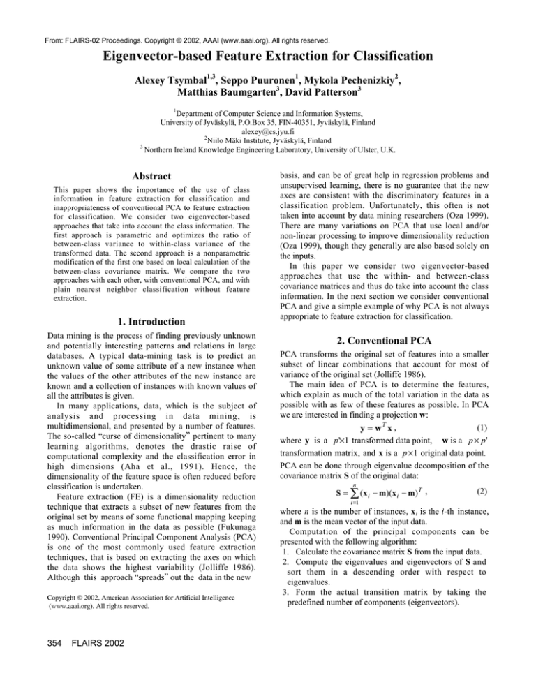
Figure 1 one can see why it can be dangerous not to use the
class information (Oza 1999). The first case shows the
proper work of PCA where the first principal component
corresponds to the variable with the highest discriminating
power, but from the second case one can see that the
chosen principal component is not always good for class
discrimination.
x2
x2
y1
y2
x1
a)
y2
y1
b)
x1
Fig. 1. PCA for classification: a) effective work of PCA, b) an
irrelevant principal component was chosen wrt. to classification.
Nevertheless, conventional PCA is still often applied to
feature extraction for classification by researchers.
3. Parametric Eigenvalue-based FE
Feature extraction for classification is a search among all
possible transformations for the best one, which preserves
class separability as much as possible in the space with the
lowest possible dimensionality (Aladjem, 1994). The usual
decision is to use some class separability criterion, based
on a family of functions of scatter matrices: the withinclass covariance, the between-class covariance, and the
total covariance matrices.
The within-class covariance matrix shows the scatter of
samples around their respective class expected vectors:
c
ni
i =1
j =1
SW =  ni  (x (ji ) - m (i ) )(x (ji ) - m (i ) ) T ,
(3)
where c is the number of classes, n i is the number of
instances in a class i, x (ij ) is the j-th instance of i-th class,
and m(i) is the mean vector of the instances of i-th class.
The between-class covariance matrix shows the scatter
of the expected vectors around the mixture mean:
c
S B = Â ni (m (i ) - m)(m (i ) - m) T ,
(4)
i =1
where c is the number of classes, n i is the number of
instances in a class i, m (i) is the mean vector of the
instances of i-th class, and m is the mean vector of all the
input data.
The total covariance matrix shows the scatter of all
samples around the mixture mean. It can be shown
analytically that this matrix is equal to the sum of the
within-class and between-class covariance matrices
(Fukunaga 1990):
(5)
S = S B + SW .
One possible criterion based on the between- and
within-class covariance matrices (3) and (4) to be
optimized for feature extraction transformation (1) is
defined in Fisher linear discriminant analysis:
wT S w
(6)
J (w ) = T B .
w SW w
A number of other criteria were proposed in (Fukunaga
1990). The criterion (6) and some other relevant criteria
may be optimized by the following algorithm often called
simultaneous diagonalization (Fukunaga 1990):
1. Transformation of X to Y: Y = Ë -1/2Ö T X , where Ë
and Ö are the eigenvalues and eigenvectors
matrices of S W .
2. Computation of S B in the obtained Y space.
3. Selection of m eigenvectors of S B , ø 1,..., ø m , which
correspond to the m largest eigenvalues.
4. Finally, new feature space Z = ØTm Y , where
Ø = [ø 1,..., ø m ] , can be obtained.
It should be noted that there is a fundamental problem
with the parametric nature of the covariance matrices. The
features extracted with the parametric approach are
suboptimal in the Bayes sense. The rank of the betweenclass covariance matrix (4) is at most c-1 (because it is the
summation of c rank one matrices and only c-1 of them are
independent), and hence no more than c -1 of the
eigenvalues will be nonzero. The nonparametric method
for feature extraction overcomes the above-mentioned
problem.
4. Nonparametric Eigenvalue-based FE
The nonparametric method tries to increase the number of
degrees of freedom in the between-class covariance matrix
(4), measuring the between-class covariances on a local
basis. K-nearest neighbor (kNN) technique is used for this
purpose.
A two-class nonparametric feature extraction method
was considered in (Fukunaga 1990), and it is extended in
this paper to the multiclass case. The algorithm for
FLAIRS 2002
355
nonparametric feature extraction is the same as for the
parametric extraction (Section 3). Simultaneous
diagonalization is used as well, and the difference is only
in calculation of the between-class covariance matrix. In
the nonparametric between-class covariance matrix, the
scatter of the samples around the expected vectors of other
classes’ instances in the neighborhood is calculated:
ni
c
c
( j)
(i )
( j) T ,
S B =  ni  wik  (x (ki ) - m ik
* )(x k - m ik * )
i =1
where
m ik( j*)
k =1
(7)
j =1
j πi
is the mean vector of the nNN instances of j-th
x (ik )
class, which are nearest neighbors to
. The number of
nearest instances nNN is a parameter, which should be set
in advance. In (Fukunaga 1990) it was proposed to use
n N N equal to 3, but without any justification. The
coefficient wik is a weighting coefficient, which shows
importance of each summand in (7). The goal of this
coefficient is to assign more weight to those elements of
the matrix, which involve instances lying near the class
boundaries and thus more important for classification. We
generalize the two-class version of this coefficient
proposed in (Fukunaga 1990) to the multiclass case:
wik =
j)
min j {d a (x (ki ) , x (nNN
)} ,
c
Âd
j =1
a
j)
(x (ki ) , x (nNN
(8)
)
(i )
j)
where d (x (ki ) , x (nNN
) is the distance from x k to its nNNnearest neighbor of class j, and a is a parameter which
should be set in advance. In (Fukunaga 1990) the
parameter a equal to 1 was used, but without any
justification.
In the next section we consider our experiments where
we analyze and compare the described above featureextraction techniques.
5. Experiments
The experiments were conducted on 21 data sets with
different characteristics taken from the UCI machine
learning repository (Blake et al., 1998). The main
characteristics of the data sets are presented in Table 1,
which includes the names of the data sets, the numbers of
instances included in the data sets, the numbers of different
classes of instances, and the numbers of different kinds of
features (categorical and numerical) included in the
instances. The pre-selected values for the a and nNN are
included in the table as well. In (Tsymbal et al., 2001) we
have presented results of experiments with several feature
selection techniques on these data sets.
In the experiments, the accuracy of 3-nearest neighbor
classification based on the heterogeneous Euclideanoverlap metric was measured to test the feature extraction
approaches. Categorical features were binarized as it was
356
FLAIRS 2002
done in the correlation-based feature selection experiments
in (Hall et al., 2000). Each categorical feature was replaced
with a redundant set of binary features, each corresponding
to a value of the original feature.
Table 1. Characteristics of the data sets
Data set
Instances
Classes
Balance
Breast
Car
Diabetes
Glass
Heart
Ionosphere
Iris Plants
LED
LED17
Liver
Lymph
MONK-1
MONK-2
MONK-3
Soybean
Thyroid
Tic-Tac-Toe
Vehicle
Voting
Zoo
625
286
1728
768
214
270
351
150
300
300
345
148
432
432
432
47
215
958
846
435
101
3
2
4
2
6
2
2
3
10
10
2
4
2
2
2
4
3
2
4
2
7
Features
Categorical
0
9
6
0
0
0
0
0
7
24
0
15
6
6
6
0
0
9
0
16
16
Numerical
4
0
0
8
9
13
34
4
0
0
6
3
0
0
0
35
5
0
18
0
0
a
nNN
1/3
255
5
1
5
63
1/5
127
1
1
1
31
3
255
1/5
31
1/3
15
5
15
3
7
1
7
1
1
20
63
1/3
1
1
3
3
215
1
1
3
3
1/3
15
1/20
7
For each data set 70 test runs of Monte-Carlo cross
validation were made, first, to select the best a and nNN
parameters, and after to evaluate the classification accuracy
with the three feature extraction approaches and without
any feature extraction. In each run, the data set is first split
into the training set and the test set by stratified random
sampling to keep class distributions approximately same.
Each time 30 percent instances of the data set are first
randomly picked up to the test set. The remaining 70
percent instances form the training set, which is used for
finding the feature-extraction transformation matrix (1).
The test environment was implemented within the MLC++
framework (the machine learning library in C++) (Kohavi
et al. 1996).
First, a series of experiments were conducted to select
the best a and nNN coefficients for the nonparametric
approach. The parameter a was selected from the set of 9
values: a Π{1 / 20, 1 / 10, 1 / 5, 1 / 3, 1, 3, 5, 10, 20}, and the
number of nearest neighbors nNN from the set of 8 values:
nNN = 2 i - 1, i = 1,...,8 , nNN Π{1, 3, 7, 15, 31, 63, 127, 255}.
The parameters were selected on the wrapper-like basis,
optimizing the classification accuracy. For some data sets,
e.g. LED and LED17, selection of the best parameters did
not give almost any improvement in comparison with the
considered in (Fukunaga 1990) a =1 and nNN=3, and the
classification accuracy varied within the range of one
percent. It is necessary to note that the selection of the
a and nNN parameters changed the ranking of the three
feature extraction approaches from the accuracy point of
view only on two data sets, thus demonstrating that the
nonparametric approach is robust wrt. the built-in
parameters. However, for some data sets the selection of
the parameters had a significant positive effect on the
classification accuracy. For example, on the MONK-2 data
set, accuracy is 0.796 when a =1 and nNN=3, but it
reaches 0.974 when a =20 and nNN=63.
After, we have compared four classification techniques:
the first three were based on the three considered above
feature extraction approaches, and the last one did not use
any feature extraction. For each feature selection
technique, we have considered experiments with the best
eigenvalue threshold of the following set {0.65, 0.75, 0.85,
0.9, 0.95, 0.97, 0.99, 0.995, 0.999, 1}.
The basic results of the experiments are presented in
Table 2. First, average classification accuracies are given
for the three extraction techniques: PCA, the parametric
(Par) and nonparametric (NPar) feature extraction, and no
feature extraction (Plain). The bold-faced and underlined
accuracies represent the approaches that were significantly
better than all the other approaches; the bold-faced only
accuracies represent the approaches that were significantly
worse on the corresponding data sets (according to the
Student t-test with 0.95 level of significance). Then, the
corresponding average numbers of extracted features are
given. The remaining part contains the average extraction
and the total expended time (in seconds) for the
classification techniques. All the results are averaged over
the 70 Monte-Carlo cross-validation runs.
Each row of Table 2 corresponds to one data set. The
last two rows include the results averaged over all the data
sets (the last row), and over the data sets containing
categorical features (the row before the last one).
From Table 2 one can see that the nonparametric
approach has the best accuracy on average (0.824).
Comparing the total average accuracy with the average
accuracy on the categorical data sets, one can see that the
nonparametric approach performs much better on the
categorical data, improving the accuracy of the other
approaches (as on the MONK data sets, and the Tic-TacToe data set). The parametric approach is the second best.
As we supposed, it is quite unstable, and not robust to
different data sets’ characteristics (as on the MONK-1,2
and Glass data sets). The case with no feature selection has
the worst average accuracy.
The parametric approach extracts the least number of
features on average (only 2.3), and it is the least timeconsuming approach. The nonparametric approach is able
to extract more features due to its nonparametric nature
(9.9 on average), and still it is less time-consuming than
the PCA and Plain classification.
Still, it is necessary to note that each feature extraction
technique was significantly worse than all the other
techniques at least on one data set (e.g., the Heart data set
for the nonparametric approach), and it is a question for
further research to define the dependencies between the
characteristics of a data set and the type and parameters of
the feature extraction approach best suited for it. For each
data set, we have also pairwise compared each feature
extraction technique with the others using the paired
Table 2. Results of the experiments
Data set
Accuracy
Features
Extraction time, sec.
Total time, sec.
PCA
.827
.721
.824
.730
.659
.777
.872
.963
.646
.395
.664
.813
.767
.717
.939
.992
.921
.971
.753
.923
.937
Par
.893
.676
.968
.725
.577
.806
.843
.980
.630
.493
.612
.832
.687
.654
.990
.987
.942
.977
.752
.949
.885
NPar
.863
.676
.964
.722
.598
.706
.844
.980
.635
.467
.604
.827
.952
.962
.990
.986
.933
.984
.778
.946
.888
Plain
.834
.724
.806
.730
.664
.790
.849
.955
.667
.378
.616
.814
.758
.504
.843
.995
.938
.684
.694
.921
.932
PCA
4.0
16.5
14.0
7.0
4.4
13.0
9.0
2.0
7.0
24.0
4.9
31.4
10.0
8.0
11.0
7.8
4.0
18.0
16.0
15.9
15.1
Par
1.0
1.0
3.0
1.0
5.0
1.0
1.0
1.0
7.0
6.7
1.0
3.0
1.0
1.0
1.0
1.0
2.0
1.0
3.0
1.0
6.4
NPar
2.0
33.7
6.4
3.8
9.0
4.4
2.0
1.0
7.0
11.4
3.1
32.0
2.0
2.0
1.9
2.2
2.0
2.0
12.5
61.7
6.5
Plain
4.0
51.0
21.0
8.0
9.0
13.0
34.0
4.0
14.0
48.0
6.0
47.0
17.0
17.0
17.0
35.0
5.0
27.0
18.0
82.0
36.0
PCA
.00
2.66
.38
.22
.11
.13
1.52
.01
.13
1.88
.06
1.58
.39
.40
.37
.17
.05
.80
.55
3.37
.62
Par
.09
3.10
.53
.24
.08
.23
1.50
.05
.39
2.46
.15
2.04
.55
.60
.55
.45
.03
.96
.53
4.29
.85
Npar
.21
4.00
.64
.30
.13
.31
2.08
.04
.49
3.10
.15
2.50
.67
.70
.69
.44
.05
1.21
.67
5.76
1.09
PCA
3.11
5.33
12.02
6.73
.69
2.63
3.49
.03
1.61
5.66
1.65
3.39
4.47
3.76
4.89
.23
.52
11.45
10.34
5.56
1.03
Par
1.02
3.31
3.08
1.38
.69
.44
1.77
.13
1.92
3.54
.53
2.23
1.06
1.08
1.07
.46
.35
1.68
2.39
4.46
1.00
NPar
1.87
9.32
6.43
4.15
1.19
1.21
2.55
.08
1.99
4.91
1.17
4.39
1.57
1.60
1.54
.47
.33
2.50
8.02
14.05
1.28
Plain
2.55
5.88
12.07
7.14
1.01
2.14
6.09
.20
2.17
5.48
1.88
1.96
4.94
4.96
4.94
.07
.69
11.24
10.42
7.88
.78
Average (categoric)
.787
.795
.845
.730
15.5
2.9
15.1
34.3
1.14
1.48
1.90
5.38
2.22
4.51
5.66
Average (total)
.801
.803
.824
.766
11.6
2.3
9.9
24.4
.73
.94
1.20
4.22
1.60
3.36
4.50
Balance
Breast
Car
Diabetes
Glass
Heart
Ionospher
Iris
LED
LED17
Liver
Lymph
MONK-1
MONK-2
MONK-3
Soybean
Thyroid
TicTacToe
Vehicle
Voting
Zoo
FLAIRS 2002
357
Student t-test with 0.95 level of significance. Results of the
comparison are given in Table 3. Columns 2-5 of the table
contain results of the comparison of the technique
corresponding to the row of the cell against the technique
corresponding to the column using the paired t-test.
Each cell contains win/tie/loss information according to
the t-test, and in parenthesis the same results are given for
the eleven data sets including categorical features. For
example, PCA has 8 wins against the parametric extraction
on 21 data sets, and 5 of them are on categorical data sets.
Table 3. Results of the paired t-test (win/tie/loss information)
PCA
PCA
Parametric
Nonparametric
Plain
10/3/8
(6/0/5)
13/1/8
(8/0/3)
4/8/9
(1/5/5)
Parametric
Nonparametric
Plain
8/3/10
(5/0/6)
8/1/13
(3/0/8)
5/11/5
(2/6/3)
9/8/4
(5/5/1)
11/5/5
(7/0/4)
11/3/8
(8/0/3)
5/11/5
(3/6/2)
5/5/11
(4/0/7)
8/3/11
(3/0/8)
From Tables 1, 2 one can see that classification without
feature extraction is clearly the worst technique even for
such data sets with relatively small numbers of features.
This shows the so-called “curse of dimensionality” and
necessity in feature extraction.
According to Table 3, among the three feature extraction
techniques, the parametric and nonparametric techniques
are the best on average, with the nonparametric technique
being only slightly better than the parametric (3 wins
versus 2 on the categorical data sets).
Conventional PCA was the worst feature extraction
technique on average, which supports our expectations, as
it does not take into account the class information.
However, it was surprisingly stable. It was the best
technique only on four data sets, but it was still the worst
one only on three data sets (the best result).
On the categorical data sets the results are almost the
same as on the rest of data sets. Only the nonparametric
technique performs much better on the categorical data for
this selection of the data sets, however, further experiments
are necessary to check this finding.
6. Conclusions
PCA-based techniques are widely used for classification
problems, though they generally do not take into account
the class information and are based solely on inputs.
Although this approach can be of great help in
unsupervised learning, there is no guarantee that the new
axes are consistent with the discriminatory features in a
classification problem.
The experimental results supported our expectations.
Classification without feature extraction was clearly the
worst. This shows the so-called “curse of dimensionality”
and necessity in feature extraction. Conventional PCA was
the worst feature extraction technique on average and,
358
FLAIRS 2002
therefore, cannot be recommended for finding features that
are useful for classification. The nonparametric technique
was only slightly better than the parametric one on
average. However, this can be explained by the selection of
the data sets, which are relatively easy to learn and do not
include significant nonnormal class distributions. Besides,
better parameter tuning can be used to achieve better
results with the nonparametric technique. This is an
interesting topic for further research. The nonparametric
technique performed much better on the categorical data
for this selection of the data sets, however, further research
is necessary to check this finding.
Another important topic for further research is to define
the dependencies between the characteristics of a data set
and the type and parameters of the feature extraction
approach best suited for it.
Acknowledgements. This research is partly supported by
the COMAS Graduate School of the University of
Jyväskylä, Finland and NEURE project of Niilo Mäki
Institute, Finland. We would like to thank the UCI ML
repository of databases, domain theories and data
generators for the data sets, and the MLC++ library for the
source code used in this study.
References
Aha, D., Kibler, D., Albert, M. 1991. Instance-based
learning algorithms. Machine Learning, 6:37-66.
Aladjem, M. 1994. Multiclass discriminant mappings.
Signal Processing, 35:1-18.
Blake, C.L., Merz, C.J. 1998. UCI Repository of Machine
Learning Databases [http:// www.ics.uci.edu/ ~mlearn/
MLRepository.html]. Dept. of Information and Computer
Science, University of California, Irvine CA.
Fukunaga, K. 1990. Introduction to Statistical Pattern
Recognition. Academic Press, London.
Hall, M.A. 2000. Correlation-based feature selection of
discrete and numeric class machine learning. In Proc. Int.
Conf. On Machine Learning (ICML-2000), San Francisco,
CA. Morgan Kaufmann, San Francisco, CA, 359-366.
Jolliffe, I.T. 1986. Principal Component Analysis.
Springer, New York, NY.
Kohavi, R., Sommerfield, D., Dougherty, J. 1996. Data
mining using MLC++: a machine learning library in C++.
Tools with Artificial Intelligence, IEEE CS Press, 234-245.
Oza, N.C., Tumer, K. 1999. Dimensionality Reduction
Through Classifier Ensembles. Technical Report NASAARC-IC-1999-124, Computational Sciences Division,
NASA Ames Research Center, Moffett Field, CA.
Tsymbal A., Puuronen S., Skrypnyk I., 2001. Ensemble
feature selection with dynamic integration of classifiers, In:
Int. ICSC Congress on Computational Intelligence
Methods and Applications CIMA’2001, Bangor, Wales,
U.K.