Adaptive estimation of parameters using partial
information of desired outputs
Joby Joseph and K V S Hari
ECE Department, IISc, Bangalore, 560012
India
d(n)
A general framework for forming an adaptive
algorithm for problems where only partial inforx(n)
y(n)
mation about the desired output is available, is
f(x, θ)
proposed. Based on preliminary analysis it can
e(n)
be shown that this framework can be used to efθ (n)
Error Correction
ficiently choose deep, narrow minima when there
based on partial
are many local minima. For problems like sepainformation and
ration of instantaneous mixtures (Independent
previous corrections
Component Analysis, ICA) and separation of
convolutive mixtures when cast in the proposed
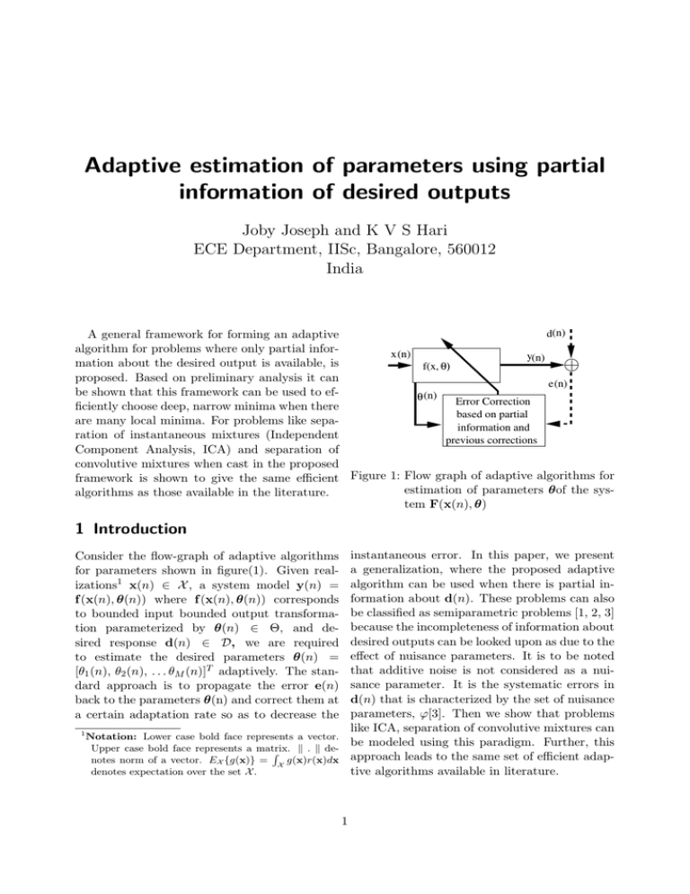
framework is shown to give the same efficient Figure 1: Flow graph of adaptive algorithms for
estimation of parameters θof the sysalgorithms as those available in the literature.
tem F(x(n), θ)
1 Introduction
instantaneous error. In this paper, we present
a generalization, where the proposed adaptive
algorithm can be used when there is partial information about d(n). These problems can also
be classified as semiparametric problems [1, 2, 3]
because the incompleteness of information about
desired outputs can be looked upon as due to the
effect of nuisance parameters. It is to be noted
that additive noise is not considered as a nuisance parameter. It is the systematic errors in
d(n) that is characterized by the set of nuisance
parameters, ϕ[3]. Then we show that problems
like ICA, separation of convolutive mixtures can
1
Notation: Lower case bold face represents a vector.
be modeled using this paradigm. Further, this
Upper case bold face represents a matrix.
k . k deR
notes norm of a vector. EX {g(x)} = X g(x)r(x)dx approach leads to the same set of efficient adapdenotes expectation over the set X .
tive algorithms available in literature.
Consider the flow-graph of adaptive algorithms
for parameters shown in figure(1). Given realizations1 x(n) ∈ X , a system model y(n) =
f (x(n), θ(n)) where f (x(n), θ(n)) corresponds
to bounded input bounded output transformation parameterized by θ(n) ∈ Θ, and desired response d(n) ∈ D, we are required
to estimate the desired parameters θ(n) =
[θ1 (n), θ2 (n), . . . θM (n)]T adaptively. The standard approach is to propagate the error e(n)
back to the parameters θ(n) and correct them at
a certain adaptation rate so as to decrease the
1
2 The adaptive algorithm
framework
able that average direction of the corrections so
far, θ, represents the right direction for this term
∆θ. Therefore ∆θ = α∆θ the average correction direction at the nth instant. Thus under
availability of partial information the stochastic
gradient descent adaptive scheme is modified to
do the corrections when ever and where ever information is available about d(n) or else assume
that the previous corrections were in the right
direction and do a weighted correction in those
directions. This modified adaptive framework is
as follows:
In the normal cases of adaptive algorithms where
d(n) is known, except for the additive noise,
θ(n) is adapted to decrease the magnitude of
the instantaneous error e(n) = d(n) − y(n).
This error measure may be any positive function E(x, θ), of e(n), E(x, θ) =k e(n) k being an
example suitable for some problems. Here it is
assumed that the error E(x, θ) is a smooth function of θ. The correction term for elements of
θ(n) is calculated by propagating the error to
the parameters θ(n) of f (x(n), θ(n)) [4] as.
∂E
|
+α(n)θ(n)
∂θ x(n),θ (n)
(2)
2 of the instan∂E
Here
µ(n)
is
the
adaptation
rate
θ(n + 1) = θ(n) − µ(n)
|x(n),θ(n)
(1)
∂θ
taneous error, and α(n) is that of the term due
to all previous adaptations(ie. memory). Let
∂E
Here µ(n) is the adaptation rate, ∂ θ is β(n) = µ(n)/α(n). Then equation(2) can be
∂E ∂E
∂E T
[ ∂θ
. . . ∂θ
] . Equation (1) minimizes an written as
1 ∂θ2
N
approximation to the cost-function CX (θ) =
∂E
|
+α(n)θ(n) (3)
θ(n + 1) = θ(n) − β(n)α(n)
∂θ x(n),θ (n)
EX {E(x|θ)} with respect to θ. Given θ, the
function Eθ (x) characterizes the errors that can
Remarks:
occur for various x. At the optimum θ = θ opt ,
• We can interpret α(n)θ(n) as the memory
C(θ) = 0 and J = cov(E(x|θ)) has finite eigenterm and −α(n)β(n) ∂∂Eθ |x(n),θ (n) as the invalues.
stantaneous error correction term.
Consider the case where d(n) is not available, for then equation(1) cannot be used. In
• Denoting the j th element of E, as Ej , we
some cases, partial information about d(n) is
∂E
propose that ∂θji can be set to zero when
available, like, for example, d(n) ∈ Rm , d(n)
there is no information available to compute
is known for some n and unknown otherwise,
it.
elements of d(n) are independent, elements of
d(n) are distributed as some r(.). Using such
• For convergence in mean it is required that
partial information, ∂∂Eθ |x(n),θ(n) can be apE{θ(n + 1) − θ(n)} = 0. For this to be
proximated. Define the set Xe (θ) = {x :
satisfied
y such that is possibly correct}. Let Xe0 (θ) be
∂E
the complement of the set of Xe (θ), ie. set of x
lim E{−α(n)β(n)
|
+α(n)θ(n)} = 0
n→∞
∂θ x(n),θ (n)
such that y is definitely in error. If adaptation
framework in (1) is used then on convergence
• For stability, variance of the correction
it would have minimized an approximation to
term, J(n) = var{−α(n)β(n) ∂∂Eθ |x(n),θ (n)
the cost CX 0 e (θ) = EX 0 e {E(x|θ)} rather than
+α(n)θ(n)} should converge to a constant
CX (θ). This is because equation (1) prevents
finite value J(∞). Thus the correction term
the freedom to explore of the elements of the pa∂y
rameter set Θ around the converged value after 2 If y is a scalar and x is a vector then ∂x
∂y
∂y
∂y T
=[ ∂x1 ∂x2 . . . ∂xN ] . If y and x are vectors then
convergence. To facilitate this exploration we
∂y
can add a ∆θ factor to equation (1). Because
ijth element of the matrix ∂y
is ∂xji . EX {g(x)} =
∂x
R
g(x)r(x)dx denotes expectation over the set X .
CX (θ) is assumed to be smooth it is more probX
θ(n + 1) = θ(n) − µ(n)
2
n−2
X 2
can be interpreted as an estimating funcδθ(n) =θ(n) − θ(n − 1) = (1 + α0 )n−1 α0 θ(0) −
α0
tion[5].
i=0
i
∂E
∂E
|
−α0 β0
|
(6)
(1 + α0 ) β0
• For the case where full information about
∂θ x(n−i),θ (n−i)
∂θ x(n),θ (n)
d(n)is available, to make the algorithm
Thus the adaptation term at any time n is havin equation (3) reduce to the conventional
ing three terms.
stochastic gradient algorithm we have to
make α(n) → 0 and β(n) → ∞ so that
1. −α0 β0 ∂∂Eθ |x(n),θ (n) corresponds to the inβ(n)α(n) is finite. β(n) has to be adstantaneous adaptation term.
justed to make the algorithm stable and
P
∂E
2
i
2. − n−2
can be even data depended, as in the case
i=0 α0 (1+α0 ) β0 ∂ θ |x(n−i),θ (n−i) corresponds to the memory term. It is the global
of learning parameter of Normalized Least
direction inferred from all the past correcMean Squared (NLMS) algorithm. It is not
tions based on the errors available. For all
possible to say about the choice of α(n)
the past corrections to be weighted equally,
and β(n) nor the stability of the adaptaα0 → 0 and simultaneously β0 → ∞ for the
tion algorithm without knowing structure
learning rate α0 β0 to be finite.
of f (x(n), θ) which is specific to an application.
3. (1 + α0 )n−1 α0 θ(0) corresponds to the initialization. This would produce a biased es• You may notice that this is similar to but
not identical to the momentum method
timate. For this factor to vanish θ(0) has to
proposed by Rumelhart et al.[6], see
be set to 0. But some problems would reequation(4), in a context other than with
quire that θ(0) be nonzero for the iteration
only partial information.
to start moving.
θ(n+1) = θ(n)−β(n)α(n)
∂E
|
+α(n)(θ(n)−θ(n−1))
∂θ x(n),θ (n)
(4) Behavior
near the optimum, θ opt
Assume E to be quadratic in e near θ opt , which
In equation(2) if we replace α(n)θ(n) with implies that on convergence to θ
conv ,
α(n)(θ(n) − θ(0)) we can compare it with
the momentum method and see the differ- ∂E |x(n),θconv = κe(n) = κ (f (x(n), θopt ) − f (x(n), θconv ))
∂e
ence. While in momentum method only
T
T
∂f
∂f
dθ =
(θ opt − θ conv ) (7)
= df =
the immediate past adaptation is used, pro∂θ
∂θ
posed method uses the entire past history
where κ is some constant. This implies
of θ to do the present adaptation and thus
can capture the average direction of descend
T
T
∂E
∂e ∂E
∂f
∂E
∂f
∂f
|x(n),θ conv =
=
=
dθ
when only partial error information is avail∂θ
∂θ ∂e
∂θ
∂e
∂θ
∂θ
able for correction.
= R̂ (θ(n), x(n)) (θ
−θ )
(8)
conv
f
opt
T
∂f
where R̂f (θ(n), x(n)) = ∂∂fθ
. There∂θ
fore when θ(n)is in the neighborhood of θ opt ,
3 Properties of the proposed
framework
θ conv = θ conv +α(n)θ conv −β(n)α(n)R̂f (θ conv , x(n))(θ conv −θ)opt )
(9)
Convergence behavior
Substituting recursively for θ(n) in equation On convergence θ(n + 1) = θ(n) = θ conv which
(3), and assuming α(n) = α0 , β(n) = β0 con- is possible if
stants,
n
θ(n) = (1 + α0 ) θ(0) −
n−1
X
i=0
∂E
α0 β0
|
∂θ x(n),θ (n)
E α(n)θ conv + θ conv β(n)α(n)R̂f (θ conv , x(n))
(5)
= E θ opt β(n)α(n)R̂f (θ conv , x(n))
3
(10)
Therefore on convergence
where αand β have been chosen to be constants.
The fact that si are independent implies that
corrections to each parameter affecting si can
be done independently. Define ei (n) as
θ conv = θ opt E β(n)R̂f (θ conv , x(n))
−1
I + E β(n)R̂f (θ conv , x(n))
=
−1
θ opt E β(n)R̂f (θ conv , x(n))
−1
+ I (11)
(
ei (n) =
The adaptive framework
n make θ converge to
o a
value near to θ opt if E β(n)R̂f (θ(n), x(n)) is
full rank and has large norm. This implies that
this approach can be used to choose the minima
with such a property, ie. deep narrow minima,
from among all the local minima. Also we can
infer that for the case where the proposed method
reverts to the standard gradient descent, which
happens when β → ∞ and α → 0, for θ to converge to θ opt we need R̂f (θ conv , x(n)) to be full
rank . The proposed framework will be studied
further with the help of a few applications in the
following sections.
ˆ (n)| > γ
−ŝi (n)/|ŝi (n)| if |s
i
0 otherwise
Form the vector e(n) = [e1 (n) e2 (n) . . . eM (n)]T .
The gradient ∂yi /∂Wij = xj , and therefore ∂E/∂Wij = ei ∂yi /∂Wij = ei xj , assum∂E
ing quadratic E . Therefore ∂W
|x(n),W(n) =
T
e(n)x (n).
Using natural gradient to orthogonalize the corrections[9], the correction factor becomes e(n)xT (n)WT (n)W(n) =
e(n)yT (n)W(n). Therefore equation (12) becomes
W(n + 1)
=
W(n) + αW(n) + βαe(n)yT (n)W(n)
=
W(n) + α(I + βe(n)yT (n))W(n)
which is the adaptation algorithm arrive at
in [7, 10, 11, 12, 13]. The work [13] shows the
4 Application of the algorithm to above error function which is the replacement of
nonlinearity in [13] is stable for any continuous,
various problems
symmetric, differentiable, non-gaussian r(.).
Remark: This example demonstrates that
4.1 Blind separation of instantaneous
using
equation (3) we can obtain the adaptalinear mixtures
tion rule which was originally derived starting
Here the measurements available are x(n) = a maximum likelihood(ML) cost function[7, 10,
As(n), x(n) = [x1 (n) x2 (n) . . . xM (n)]T , 11, 12, 13].
s(n) = [s1 (n) s2 (n) . . . sM (n)]T whose elements si are distributed with unknown non4.2 Blind separation of convolutive
gaussian density function r(s) are independent
mixtures
[7, 8] and A is an M × M matrix whose elements are Aij . The problem is to estimate A Here the measurements available are
such that y(n) = A−1 x(n) = ŝ(n) , an estimate
of d(n) = s(n). This problem is also known
as Independent Component Analysis (ICA). The
information we know about desired output d(n)
is that its elements are iid non-gaussian random
variables. Since nothing else is known about the
random variables it is proposed to assume as distributed uniformly with in the interval −γ to γ.
Using equation (2) it is possible to write down
the adaptation algorithm for this case.
W(n + 1) = W(n) + αW(n) + βα
∂E
|x(n),W(n)
∂W
x(n) =
P
X
p=0
B(p)s(n − p) +
Q
X
A(p)x(n − p) = B(z)A−1 (z)s(n)
q=1
where x(n) and s(n) are as defined previously
and A(z) and B(z) are matrix polynomials.
It is required to find W(z) such that y(n) =
W(z)x(n) = s(n) have independent elements.
The adaptation algorithm would be in the form
Wp (n + 1) = Wp (n) + αWp (n) + βα
∂E
|x(n),Wp (n)
∂Wp
(13)
where αand β are fixed constants. Since the
information available about the source density
(12) is the same as in the instantaneous mixture case
4
per turns out to be the same. The method gives
a way of using the known information efficiently
unlike in other cases where this is left to be in
the form of an unknown nonlinearity. This approach can be used to choose the minima with
such a property, ie. deep narrow minima, from
Wp (n) + αWp (n)+
among all the local minima. We are working on
Wp (n + 1) =
βαe(n)xT (n − p)WT (z −1 )W(z)
finding, for what class of f (x, θ) is equation (3)
Remark: Using equation (3) we could arrive at applicable and how to choose α and β.
the same algorithm derived starting from a ML
cost function in [2, 10, 11].
the error function is the same. Following the
same line of argument as in the instantaneous
∂E
mixture case, ∂W
= e(n)xT (n − p). Using the
p
fact that the elements of s(n) are independent
and by applying natural gradient to the error
correction
References
5 Discussion
[1] Shun-Ichi Amari and Jean-Francois Cardoso, “Blind source separation — semiparametric statistical approach,” IEEE Transaction on SP, pp. –, 1997.
In the above examples application of the general
principle (2) to problems with partial information on desired output led to identical algorithms
as derived using various approaches in the existing literature in two cases of source separation.
This approach gives a clue as to how possibly
the available information about the nuisance parameter can be used to form adaptive estimators. But once having formulated the algorithm
it can be explained in various ways following
other works in the literature. For example in the
case of ICA because the error function e() is nonlinear it can be expanded in terms of powers of
si and hence the adaptation algorithm minimizes
the cross cumulants of the recovered signals. Another way to interpret is that the algorithm minimizes marginal mismatch since the information
about r(si ) used is that about the marginal densities. Since adaptation term is formed assuming
independence of sources we can say that it corrects for deviation from independence.
[2] L.-Q. Zhang, S. Amari, and Cichocki, Advances in Neural Information Processing
12, MIT Press, 2000.
[3] Shun ichi Amari and Motoaki Kawanabe,
“Information geometry of estimating functions in semiparametric statistical models,”
Bernouli, vol. 2, no. 3, pp. –.
[4] Simon Haykins, Adaptive Filter Theory,
Prentice-Hall International, Inc, first edition, 1996.
[5] S. Amari and M. Kawanabe, “Estimating functions in semiparametric statistical
model,” Selected Proceedings of the Symposium on Estimating Functions, IMS Lecture
Notes–Monograph Series, vol. 32, pp. 65–81,
1997.
[6] D. Rumelhart, G. Hinton, and R. Williams,
Parallel Distributed Processing, MIT Press,
1986.
6 Conclusion
The current work shows a practical framework for forming adaptive algorithms for problems where some partial information is available
about the desired output. In two cases where in
the literature algorithms have been formed using
different approaches like estimating function and
maximum likelihood method, the adaptive algorithms constructed using the principle in this pa-
[7] Jean-Francois Cardoso, C. N. R. S., and
E. N. S. T., “Blind signal separation: Statistical principles,” Proceeedings of IEEE, vol.
86, no. 10, pp. 2009–2025, October 1998.
[8] Pierre Comon, “Independent component
analysis, a new concept?,” Signal Processing, vol. 36, pp. 287–314, 1994.
5
[9] Shun ichi Amari, “Natural gradient works
efficiently in learning,” Neural Computation, vol. 10, no. 2, pp. 251–276, 1998.
[10] Shun ichi Amari, Scott C. Douglas, Andrzej
Cichocki, and Howar H Yang, “Novel online adaptive learning algorithm for blind
deconvoution using the natural gradient approach,” pp. –.
[11] Scott C. Douglas, Andrzej, and Shun ichi
Amari, “Multichannel blind separation and
deconvolution of sources with arbitrary distributions,” IEEE workshop on Neural Networks or Signal Processing, Almelia Island
Plantation, pp. 436–445, Sept 1997.
[12] Pierre Common, Chritian Jutten, and
Jeanny Herault,
“Blind separation of
sources, part i: An adaptive algorithm
based on neuromimetic architecture,” Signal Processing, vol. 24, pp. 1–10, 1991.
[13] Heinz Mathis an Scott C. Douglas, “On
the existance of universal nonlinearities for
blind source separation,” IEEE Transaction
on SP, vol. 50, no. 5, pp. 1007–1016, May
2002.
6