6.262: Discrete Stochastic Processes
4/25/11
L20: Markov processes and Random Walks
Outline:
• Review - Steady state for MP
• Reversibility for Markov processes
• Random walks
• Queueing delay in a G/G/1 queue
• Detection, decisions, & Hypothesis testing
1
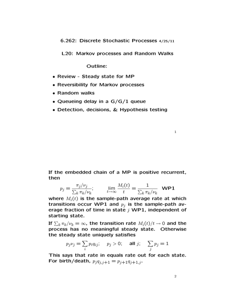
If the embedded chain of a MP is positive recurrent,
then
πj /νj
Mi(t)
1
;
lim
=�
WP1
pj = �
t→∞
t
k πk /νk
k πk /νk
where Mi(t) is the sample-path average rate at which
transitions occur WP1 and pj is the sample-path av­
erage fraction of time in state j WP1, independent of
starting state.
�
If k πk /νk = ∞, the transition rate Mi(t)/t → 0 and the
process has no meaningful steady state. Otherwise
the steady state uniquely satisfies
pj νj =
�
i
piqij ;
pj > 0;
all j;
�
pj = 1
j
This says that rate in equals rate out for each state.
For birth/death, pj qj,j+1 = pj+1qj+1,j .
2
For an irreducible process, if there is a solution to the
equations
pj νj =
�
piqij ;
pj > 0;
�
all j;
i
�
pj = 1
j
and if i νipi < ∞, then the embedded chain is positive
recurrent and
�
�
pj νj
πj = �
;
πi/νi = ( pj νj )−1
i piνi
i
i
�
If i νipi = ∞, then each πj = 0, the embedded chain
is either transient or null-recurrent, and the notion of
steady-state makes no sense.
3
✓✏
0

②
✒✑
1
0.6
2
✓✏
1
1

③
0.4
1
②

✒✑
0.4
2
0.6
2
✓✏

③
2

②
✒✑
23
✗✔

③
3
...
✖✕
0.4
Imbedded chain for hyperactive birth/death
1
1.2
2.4
✗✔
✓✏
✓✏
✓✏
0
②

✒✑

③
0.8
1

②
✒✑
③

1.6
2

②
✒✑

③
3
...
✖✕
3.2
Same process in terms of {qij }
Using pj qj,j+1 = pj+1qj+1,j , we see that pj+1 = 3
4 pj , so
�
pj = (1/4) (3/4)j and
pj νj = ∞.
j
If we truncate this process to k states, then
pj
�
j
pj νj
�
� �k � � �j
� �k � � �k−j
3
3
1
2
2
=
1−
;
πj =
1−
4
4
3
3
3
�
�
� �k � �� �k
1
3
3
=
1−
− 1 → ∞
2
4
2
1
4
�
4
Reversibility for Markov processes
For any Markov chain in steady state, the backward
∗ are defined as
transition probabilities Pij
∗ =π P
πiPij
j ji
There is nothing mysterious here, just
�
�
Pr Xn = j, Xn+1 = i
�
�
�
�
= Pr Xn+1 = i Pr Xn=j|Xn+1=i
�
= Pr{Xn = j } Pr Xn+1=i|Xn=j
�
This also holds for the embedded chain of a Markov
process.
✛
State i
✲✛
State j, rate νj
t1
✲✛
State k
✲
t2
5
✛
State i
✲✛
t1
State j, rate νj
✲✛
State k
✲
t2
Moving right, after entering state j, the exit rate is νj ,
i.e., we exit in each δ with probability νj δ. The same
holds moving left.
That is, a Poisson process is clearly reversible from
the incremental definition.
Thus {πi} and {νi} are the same going left as going
right
6
Note that the probability of having a (right) transition
∗ is
from state j to k in (t, t+δ) is pj qjk δ. Similarly, if qkj
the left-going process transition rate, the probability
∗ . Thus
of having the same transition is pk qkj
pj qjk = pk qk∗j
∗ = ν P∗ .
By fiddling equations, qkj
k kj
∗ = q for all i, j
Def: A MP is reversible if qij
ij
�
Assuming positive recurrence and i πi/νi < ∞, the MP
process is reversible if and only if the embedded chain
is.
7
The guessing theorem: Suppose a MP is irreducible
and {pi} is a set of probabilities that satisfies piqij =
�
pj qji for all i, j and satisfies i piνi < ∞.
Then (1), pi > 0 for all i, (2), pi is the sample-path
fraction of time in state i WP1, (3), the process is
reversible, and (4), the embedded chain is positive
recurrent.
�
Useful application: All birth/death processes with j pj νj <
∞ are reversible. Similarly, if the Markov graph is a
�
tree with j pj νj < ∞, the process is reversible.
8
✉
✉
a2 d1
a1
✉
✉
a3
d2
✉
d3
✉
✉
a4
d4
✉
Right moving (forward) M/M/1 pro cess
✉
d3 a4
d4
✉
✉
d2
✉
✉
a3
✉
a2
d1
✉
✉
a1
Left moving (backward) M/M/1 process
Burke’s thm: Given an M/M/1 queue in steady-state
with (arrival rate) λ < µ (departure rate),
(1) Departure process is Poisson with rate λ
(2) State X(t) is independent of departures before t
(3) For FCFS, a customer’s arrival time, given its de­
parture at t, is independent of departures before t.
9
✉
✉
a2 d1
a1
✉
✉
d3 a4
d4
✉
✉
✉
a3
d2
✉
d2
✉
✉
a3
t
d3
✉
t✉
a2
✉
a4
d1
✉
d4
✉
✉
a1
A departure at t in (right-moving) sample path is an
arrival in the M/M/1 (left-moving) sample path.
For FCFS left-moving process, departure time of ar­
rival at t depends on arrivals (and their service req.)
to the right of t; independent of arrivals to left.
For corresponding (right-moving) process, the arrival
time of that departure is independent of departures
before t.
10
Poisson
λ ✲
M/M/1
M/M/1
λ
µ1
λ
✲
✲
µ2
Consider tandem M/M/1 queues. Departures from
first are Poisson with rate λ. Assume service times
at rates µ1 and µ2, independent from queue to queue
and independent of arrivals at each.
Arrivals at queue 2 are Poisson at rate λ by Burke
and are independent of service times at 2. Thus the
second queue is M/M/1.
The states of the two systems are independent and
the time of a customer in system 1 is independent of
that in 2.
11
Random walks
Def: Let {Xi; i ≥ 1} be a sequence of IID rv’s, and let
Sn = X1 + X2 + · · · + Xn for n ≥ 1. The integer-time
stochastic process {Sn; n ≥ 1} is called a random walk,
or, specifically, the random walk based on {Xi; i ≥ 1}.
We are used to sums of IID rv’s, but here the interest
is in the process. We ask such questions as:
1) Threshold crossing: For given α > 0, what is the
probability that Sn ≥ α for at least one n ≥ 1; what
is the smallest n for which this crossing happens; and
what is the overshoot Sn − α?
2) Two thresholds: For given α > 0, β < 0, what is the
probability that {Sn; n ≥ 1 crosses α before it crosses
β, and what is the n at which the first such crossing
occurs?
12
These threshold-crossing problems are important in
studying overflow in queues, errors in digital commu­
nication systems, hypothesis testing, ruin and other
catastrophes, etc.
In many of the important applications, the relevant
probabilities are very small and the problems are known
as large deviation problems.
Moment generating functions and their use in upper
bounds on these small probabilities are important here.
We start with a brief discussion of 3 simple cases: sim­
ple random walks, integer random walks, and renewal
processes.
13
Simple random walks
A random walk (RW) {Sn; n ≥ 1}, Sn = X1 + · · · + Xn is
simple if Xn is binary with pX (1) = 1, pX (−1) = q = 1−p.
This is just a scaling variation on a Bernoulli process.
The probability that Xi = 1 for m out of n trials is
n!
pm(1 − p)n−m.
m!(n − m)!
Viewed as a Markov chain,
Pr{Sn = 2m − n} =
p
q
✓✏
−2
②
✒✑
p
③

q =1−p
✓✏
−1②

✒✑
p
q
③

✓✏
0 
②
✒✑
p
✗✔

③
p
✖✕
1
q
q
As in ‘stop when you’re ahead’

∞
 �


�
�k
p
{Sn ≥ k} =
Pr


1 − p
n=1
if p ≤ 1/2.
14
Integer RW’s (where X is an integer rv) are simi­
lar. An integer RW can also be modeled as a Markov
chain, but there might be an overshoot when crossing
a treshold and the analysis is much harder.
Renewal processes are also special cases of random
walks where X is a positive rv. When sketching sample
paths, the axes are usually reversed from RP to RW.
Walk Sn
S4 ✈
α
S1 ✈
S5 ✈
Trial n
S2 ✈ S3 ✈
S✉3
S2✉
S✉ 1
Trial n
S5✉
S✉4
N (t)
time Sn α
15
Queueing delay in a G/G/1 queue
Let {Xi; i ≥ 1} be the (IID) interarrival intervals of a
G/G/1 queue and let {Yi; i ≥ 1} be the (IID) service
requirement of each.
s3
✗
0✛
✛
s✛2
1
Arrivals s✖
✛ x2
x1
✗
✲✛
✖
y0
x3
w1
✲✛
✕
w2
✲✛
✲✛
✔
y1
✔
✲✕
✲
✛
✲✛
y2
y3
✲
✲
Departures
wn is time in queue
x2 + w2 = w1 + y1 ✲
If arrival n is queued (e.g., arrival 2 above), then
xn + wn = yn−1 + wn−1
If arrival n sees an empty queue, then wn = 0.
16
wn = yn−1 − xn + wn−1 if wn−1 + yn−1 ≥ xn else wn = 0
wn = max[wn−1 + yn−1 − xn, 0]
Since this is true for all sample paths,
Wn = max[Wn−1 + Yn−1 − Xn, 0]
Define Un = Yn−1 − Xn. Then
Wn = max[Wn−1 + Un, 0]
Without the max, {Wn; n ≥ 1} would be a random walk
based on {Ui; i ≥ 1}.
With the max, {Wn; n ≥ 1} is like a random walk, but
it resets to 0 every time it goes negative. The text
restates this in an alternative manner.
17
Detection, decisions, & Hypothesis testing
These are different names for the same thing. Given
observations, a decision must be made between a set
of alternatives.
Here we consider only binary decisions, i.e., a choice
between two hypotheses.
Consider a sample space containing a rv H (the hy­
pothesis) with 2 possible values, H = 0 and H = 1.
The PMF for H, pH (0) = p0, pH (1) = p1, is called the a
priori probabilities of H.
Assume n observations, Y1, . . . , Yn are made. These are
IID conditional on H = 0 and IID conditional on H = 1.
Assume a pdf
fY� |H (�
y | �) =
n
�
i=1
fY |H (yi | �).
18
By Baye’s law,
y} =
Pr{H=� | �
p�fY� |H (�
y | �)
y | 0) + p1fY� |H (�
y | 1)
p0fY� |H (�
.
Comparing Pr{H=0 | �
y } and Pr{H=1 | �
y },
p0fY� |H (�
y | 0)
Pr{H =0 | �
y}
=
.
y | 1)
Pr{H=1 | �
y}
p1fY� |H (�
The probability that H = � �is the correct
hypothesis,
�
� . Thus we maxi­
given the observation, is Pr H=� | Y
mize the a posteriori probability of cho
�osing correctly
�
� . This
by choosing the maximum over � of Pr H=� | Y
is called the MAP rule (maximum a posteriori proba­
bility). It requires knowing p0 and p1.
19
MIT OpenCourseWare
http://ocw.mit.edu
6.262 Discrete Stochastic Processes
Spring 2011
For information about citing these materials or our Terms of Use, visit: http://ocw.mit.edu/terms.