From: AAAI-97 Proceedings. Copyright © 1997, AAAI (www.aaai.org). All rights reserved.
ete
Murray
Shanahan
Department of Computer Science,
Queen Mary and Westfield College,
Mile End Road, London El 4NS, England.
mps@dcs.qmw.ac.uk
Abstract
This paper presents a logical account of sensor data
assimilation
in a mobile robot, based on abduction.
Unlike previous work, the present formulation
handles
sensor noise as well as motor noise. In addition,
it
incorporates two significant technical advances. The use
of determining
fluents to deal with non-determinism
obviates the need for a special form of abduction, and the
use of uncertain object boundaries alleviates a problem
with multiple explanations.
Introduction
In [Shanahan, 19961, a logical characterisation of robot
sensor data assimilation via abduction is presented. The
methodology used in that paper, as well as the present
work, comprises the following three steps. First, design a
generic logical formalism for representing and reasoning
about action, change, space and shape. Second, use this
formalism to build a theory of the robot’s relationship to
the world, that is to say, a theory describing the effect of
the robot’s actions on the world and the impact of the world
on the robot’s sensors. Third, view sensor data assimilation
as abduction with this theory. The role of abduction is to
hypothesise a collection of objects whose shapes and
locations are sufficient to explain the robot’s sensor data.
Any algorithm for deployment on the actual robot which is
provably
correct with respect to this abductive
characterisation is, in effect, a map-building algorithm.
The key features of the informatic situation confronting a
mobile robot are incompleteness, due to the robot’s limited
window on the world, and uncertainty, due to noise in its
sensors and motors. The topic of noisy motors is discussed
at length in [Shanahan, 19961. In that paper, noise is
considered as a kind of non-determinism, and a consistencybased form of abduction is used. But the treatment of
incompleteness and uncertainty is unsatisfactory for a
number of reasons. Chief among these is the profligacy of
the collection of explanations licensed by abduction for a
given stream of sensor data. Other reasons include the
difficulty of performing, or even proving properties of,
consistency-based abduction.
This paper sets out to remedy the deficiencies of the earlier
work through the provision of a cleaner and more versatile
Copyright
0 1997, American
Association
(www.aaai.org).
All rights reserved.
for Artificial
Intelligence
logical account of sensor data assimilation. To deal with
the multiple explanations problem, objects are represented
with uncertain boundaries. To cope with noise, the method
of determining fluents replaces the use of non-deterministic
trajectories in [Shanahan, 19961. This permits the use of
standard, as opposed to consistency-based, abduction.
Finally, the robot that formed the basis of the earlier work
was equipped with a very simple collection of sensors,
namely three bump switches. The robot under discussion
here has a suite of eight infra-red proximity sensors,
supplying much richer sensory input. This forces us to
confront the issue of sensor noise. (There is no sensor
noise as such with a bump switch.) Accordingly, the
present paper, unlike [Shanahan, 19961, supplies a
treatment of sensor noise as well as motor noise.
epresenting
Action
The first step in the methodology
outlined in the
introduction is the development of a generic formalism for
representing and reasoning about action, change, space and
shape. This section concerns the part of the formalism for
reasoning about action and continuous change, which is
based on the circumscriptive event calculus [Shanahan,
19971. The same formalism is employed in [Shanahan,
19961. Because this material is presented in considerable
detail elsewhere, the description here will be kept very
brief.
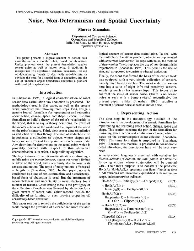
A many sorted language is assumed, with variables for
fluents, actions (or events), and time points. We have the
following axioms, whose conjunction will be denoted
CEC. Their main purpose is to constrain the predicate
HoldsAt. HoldsAt(f,t) represents that fluent f holds at time
t. All variables are universally quantified with maximum
scope, unless otherwise indicated.
HoldsAt(f,t) t- Initiallyp(f) A 1 Clipped(O,f,t)
(ECU
1 HoldsAt(f,t) t
(I33
InitiallyN(f) A T Declipped(O,f,t)
HoldsAt(f,t2) t
(EC3)
Happens(a,tl) A Initiates(a,f,tl) A
t 1 c t2 A l Clipped(t 1,f,t2)
1 HoldsAt(f,t2) t(EC4)
Happens(a,tl) A Terminates(a,f,tl) A
tl <t2A
l Declipped(t1 ,f,t2)
Clipped(tl ,f,t2) ++
(EC5)
3 a,t [Happens(a,t) A tl < t < t2 A
[Terminates(a,f,t) v Releases(a,f,t)]]
SPATIAL
UNCERTAINTY
153
non-determinism
was incorporated
into the robot’s
trajectory as it moved forwards. The present paper takes a
somewhat different approach, which I will now outline.
The method for dealing with non-determinism adopted here
involves the use of determining fluents (see [Shanahan,
1997, Chapter 15]), which are related to the noise terms
introduced for the same purpose by Poole [ 19951. With the
method of determining
fluents, actions with nondeterministic effects are transformed into actions with
deterministic effects. The trick is simply that the outcome
of an action with non-deterministic effects is made to
depend on a fluent, called a determining fluent, which
doesn’t appear elsewhere in the formalisation, and whose
value at the time of the performance of the action is
unknown. This treatment of non-determinism obviates the
need for a special form of abduction, such as the
consistency-based form of abduction used in [Shanahan,
19961. Instead, as we’ll see later on, the determining fluents
are simply made abducible.
In the formalisation of the Khepera robot, the Go and
Rotate actions have non-deterministic effects: the velocity
of the robot after a Go action is only known within certain
bounds, and the angular velocity of the robot after a Rotate
action is only known within certain bounds. In what
follows, the constant V denotes the robot’s median
velocity, measured in robot radii per unit of time, and the
constant W denotes the robot’s median angular velocity in
degrees per unit of time. The formalisation also uses the
constants ev and ew. After a Go action, the robot’s
velocity is V f Ev. Similarly, after a Rotate action, the
robot’s.angular velocity is W + zzW.
~
To capture’the effect of the Go and Rotate actions using
determining fluents, the functions VelNoise and RotNoise
are introduced. These fluents perturb the robot’s (angular)
velocity at the outset of a period of motion. If a Go action
is performed at time t, then the term VelNoise(t) denotes
the difference e, where --Ed I e I Q,, between the robot’s
actual velocity after t and the median velocity V. Similarly,
if a Rotate action is performed’ at’ time t, the term
RotNoise
denotes the difference e, where --Ed I e I Ed,
between the robot’s actual angular velocity after t and the
median angular velocity W.
We have the following Initiates and Terminates formulae,
which introduce the two new fluents Moving and Turning.
The fluent Moving(v) holds when the robot is moving at
velocity v, and the fluent Turning(w) holds when the robot
is rotating with angular velocity w.
Initiates(Go,Moving(V+VelNoise(t)),t)
(El)
Initiates(Rotate,Turning(W+RotNoise(t)),t)
(W
The following two formulae constrain the values of
VelNoise and RotNoise to fall within the required range.
-E,, < VelNoise(t) I cv
w>
-&w I RotNoise
< ~w
W)
Next, we need to define the continuous variation that takes
place in the robot’s bearing and location while,
respectively, the Turning and Moving fluents hold. The
fluent Facing(r) holds when the robot’s compass bearing is
r degrees relative to North. The fluent Location(y) holds
when the robot’s centre is at point y The continuous
variation in the Location and Facing fluents is captured by
the following Trajectory formulae.
LngW) t
Trajectory(Moving(v),t,Location(yl),
(T*)
HoldsAt(Facing(r),t) A HoldsAt(Locazon(y2),t) A
FromTo(c,y2,yl) A Bng(c,r)
Trajectory(Turning(w),t,Facing(r+d.w),d)
t
cm
HoldsAt(Facing(r),t)
After a Go action, the Location fluent is no longer subject
to default persistence. Similarly, after a Rotate action, the
Facing fluent is no longer subject to default persistence.
Releases(Go,Location(y),t)
03
Releases(Rotate,Facing(r),t)
(EA)
The following Initiates and Terminates formulae capture the
effects of the Stop action.
Terminates(Stop,Moving(v),t)
Terminates(Stop,Turning(w),t)
Initiates(Stop,Location(y),t) t
HoldsAt(Moving(v),t)
Av>0A
HoldsAt(Location(y),t)
Initiates(Stop,Facing(r),t) t
(E8)
HoldsAt(Turning(v),t) A w # 0 A
HoldsAt(Facing(r),t)
Taken in conjunction with the event calculus axioms of
Section 1, the formulae above can be used deductively for
prediction (temporal projection). Given a description of a
sequence of robot actions, the robot’s location at any given
time can be predicted within the tolerances allowed by the
non-determinism.
Let’s take a look at an example. Let M be the conjunction
of the following formulae.
Initiallyp(Location(L0))
Initiallyp(Facing(R0))
Let N be the conjunction of the following formulae.
Happens(Go, 1000)
Happens(Stop,3000)
Happens(Rotate,4000)
Happens(Stop5000)
Happens(Go,6000)
These actions are illustrated on the right of Figure 1.
In addition, we require some uniqueness-of-names axioms.
The following will suffice for now, although we will adopt
a different set in the next section.
UNA[Go, Rotate, Stop]
(3.1)
UNA[Moving, Turning, Location, Facing]
(3.2)
Let E be the conjunction of (El) to (E8). Let B be the
conjunction of,
0 the event calculus axioms CEC,
0 the background axioms (Bl) to (B4),
0 the Trajectory formulae (Tl) and (T2), and
0 the uniqueness-of-names axioms (3.1) and (3.2).
Following the prescription for overcoming the frame
problem set out in Section 1, we’re interested in the logical
consequences of the following formula, which will be
denoted C.
SPATIAL
UNCERTAINTY
155
CIRC[N ; Happens] A
CIRC[E ; Initiates, Terminates, Releases] A M A B
The logical consequences of X are expected to describe the
path of the robot. However, the non-deterministic nature of
the robot’s actions, reflecting the fact that its motors are
noisy, means that Z doesn’t fix the exact location of the
robot at any time after its first Go action. Rather, we
should expect Z to yield consequences of the form A t- I,
where A describes the robot’s location to the bounds within
which it can be known, and l? constrains the determining
fluents VelNoise and RotNoise accordingly. A will
characterise the robot’s location in terms of a graph of
curves and locations corresponding to the path the robot
followed to get there. The following proposition gives an
example.
Proposition
3.3. Let A denote the conjunction of the
following formulae, in which cl, y 1, c2, and y2 are free.
FromTo(cl,LO,y 1) A Bng(c1) = RO A
2OOO.(V- Ev) I Lng(c1) I 2OOO.(V -t Ev) A
HoldsAt(Location(y1),3000)]
FromTo(c2,yl,y2) A lOOO.(W - &w) 5
Bng(c2) - Bng(c1) I lOOO.(W + &w) A
2OOO.(V- Ev) 5 Lng(c2) 5 2OOO.(V+ E”) A
HoldsAt(Location(y2),8000)
Let I’ denote the conjunction of the following formulae, in
which cl, y 1, c2, and y2 are also free.
VelNoise( 1000) =w
RotNoise(4000)
- V
- Bng(c~&~ng(cl)
VelNoise(6000) =s
We have C,I= 3 cl,yl,c2,y2
Proof. See full paper
- W
- V
[A +- I].
4 The Effect of the World
cl
on the Robot
The formulae of the previous section describe the effect of
the robot’s actions on the world. Now we need to
characterise the way the robot’s interactions with the world
effect its sensors. Once again, noise is a big issue. This
time the noise is in the robot’s sensors, which deliver
uncertain information about the world. As before, noise is
considered as non-determinism.
Each of the Khepera’s infra-red proximity sensors supplies
an unbroken (but discretely sampled) stream of values
between 0 and 1023. A high value suggests the proximity
of an obstacle, but unsurprisingly no straightforward
functional correspondence exists between the value of a
sensor and the distance to the nearest object. As well as
being subject to random fluctuations and spikes, the value
delivered by a sensor at any time depends on the sizes,
shapes, orientations and reflective properties of the objects
within its range. So the question arises of how to extract
useful distance information from the sensor signal,
156
AUTOMATED
REASONING
A standard way would be to use a Gaussian and/or Kalman
filter. Although benefit can still be derived from prefiltering sensor signals, the approach taken in the present
paper places the burden of interpreting sensor data at a
higher level. To begin with, raw sensor data is transformed
into a sequence of sensor events. Two types of sensor event
are incorporated into the formalisation:
LatchOn and
LatchOff, which will be parameterised by the identifier of
the sensor in question. Sensor data assimilation is then
performed through abduction, whose task is to construct an
explanation of these sensor events in terms of a map of the
obstacles in the robot’s workspace.
Intuitively, a LatchOn event indicates that an object has
been encountered, while a LatchOff event indicates that the
robot has found free space. An obvious way to implement
this is to trigger a LatchOn event whenever the sensor
signal exceeds a threshold, and a LatchOff event whenever it
dips below that threshold. However, with this method, the
presence of random noise in the sensor signal gives rise to
the possibility of a flurry of LatchOn and LatchOff events
when the signal is close to the threshold value.
Accordingly, in the present approach, sensor events are
associated with two threshold values 61 and 62, where 61 >
62. When a sensor value exceeds 61 then a LatchOn event
occurs. Conversely, when the sensor value dips below 62, a
LatchOff event occurs.
The fluent High holds when the sensor signal is greater
than 61, and the fluent Low holds when the sensor signal is
less than 62. Like the LatchOn and LatchOff events, these
fluents are parameterised by the identifier of the sensor in
question. Sensors will be grouped into pairs whose values
will be aggregated, and our main concern will be with the
pair 0 and 1, which will be called the left sensor, and the
pair 4 and 5, which will be called the right sensor (see
Figure 1). The following two clauses constrain the High
and Low fluents for the left sensor.
Holds(Low(Left),t) t
033)
7 3 y,r,c,x [HoldsAt(Location(y),t) A
HoldsAt(Facing(r),t) A
HoldsAt(Boundary(x,c),t) A
Fsen(y,r-45,c) + SenNoise(Left,t) > 621
HoldsAt(High(Left),t) t
CW
HoldsAt(Location(y),t) A HoldsAt(Facing(r),t) A
HoldsAt(Boundary(x,c),t) A
F,en(y,r45,c) + SenNoise(Left,t) > Sl]
The first of these formulae describes the conditions under
which the value of the left sensor falls below 62 at time t.
First, there has to be an object whose boundary bears a
suitable relation to the position and direction of the left
sensor at t. (The term Boundary(x,c) denotes a fluent which
holds if the curve c is part of the boundary of object x.) The
influence of such an object on the value of the sensor is
given by the function Fsen, which allows us to abstract
away from the sensor’s characteristics. Fsen(y,r,c) denotes
the median value the sensor would have if located at y on a
bearing r in a world containing only the object boundary c.
This value is combined with the effect of sensor noise at
time t, given by the term SenNoise(Left,t), to yield the
actual value of the sensor.
Symmetrical formulae are required for the right sensor.
Holds(Low(Right),t) t
WI
13 y,r,c,x [HoldsAt(Location(y),t) A
HoldsAt(Facing(r),t) A
HoldsAt(Boundary(x,c),t) A
Fsen(y,r+45,c) + SenNoise(Right,t) > 621
HoldsAt(High(Right),t) t(B6)
HoldsAt(Location(y),t) A HoldsAt(Facing(r),t) A
HoldsAt(Boundary(x,c),t) A
F,,n(y,r+45,c) + SenNoise(Right,t) > 61
The SenNoise function plays a similar role to the VelNoise
and RotNoise functions. The effect of sensor noise is
assumed fall within in a certain range although, of course,
the exact amount of sensor noise at any time is unknown.
-us < SenNoise(t) < 8s
(B7)
The effects of sensor events and the conditions under which
they are triggered are given by the following formulae,
which are generic to both the left and right sensors.
Happens(LatchOn(d),t) t
(W
1 HoldsAt(On(d),t) A HoldsAt(High(d),t)
Happens(LatchOff(d),t) t(H2)
HoldsAt(On(d),t) A HoldsAt(Low(d),t)
Initiates(LatchOn(d),On(d),t)
(E9)
Terminates(LatchOff(d),On(d),t)
@lo)
The On and Off fluents ensure that LatchOn and LatchOff
events only occur when a threshold is passed.
Finally, we have two uniqueness-of-names axioms.
UNA[Go, Rotate, Stop, LatchOn, LatchOff]
@37)
UNA[Moving, Turning, Location,
(BQ
Facing, Boundary, On, High, Low]
We’re now in a position to view sensor data assimilation as
abduction. Given a sequence of sensor events, the task is to
construct an explanation of those events by postulating the
existence of objects of suitable shapes and locations. This
task is essentially abductive. Roughly speaking, if the
sequence of sensor events is represented by the formula Y,
and we are given formulae Z, representing the relationship
between the robot and the world, and AN, representing the
robot’s actions, then we are seeking a formula AM such
that,
ZAANAAM~Y.
Care must be taken when using abduction to explain
observations
in the context of actions with nondeterministic effects. The problem is that an observation in this case Y - can have a greater degree of precision
than can be explained by the occurrence of an action with a
non-deterministic
effect. However, if the method of
determining
fluents is used, this difficulty
can be
circumvented by including values for those fluents in the
explanation.
AM is, first and foremost, a map of the world in which,
because of motor and sensor noise, the boundaries of
objects are not precisely given. But because noise is treated
as non-determinism, AM will also have to contain a certain
amount of unwanted junk. This takes the form of formulae
that assign values to the determining fluents representing
the noise present in the motors and sensors. These formulae
will be stripped from AM.
Before moving on to an example, a further definition is
required. In order to rule out explanations which posit
phantom objects, we want our explanations to entail not
only the occurrence of the events in Y, but also the nonoccurrence of events not in Y. Accordingly, we will be
looking for explanations of u/ A COMP[‘u],
where
COMP[Y] is defined as follows.
Definition
4. I.
COMP[‘P] ‘def
[Happens(a,t) A [a = LatchOn
v a = LatchOff(d
-+
v [
a=ar\t=z]
(W)E
I-
where r = {(a,@ I Happens(a,z) E Y”}.
5 A Worked
cl
Example
Figure 1 shows the robot encountering a wall. After
detecting the wall, the robot rotates so that it is sideways
on to the wall, then follows it for a while until coming to
a halt. At some time during the robot’s turn, its left sensor
will detect the wall. This is the sensor event we want to
explain.
Let Ml be the conjunction of the following formulae.
Initiallyp(Location(L0))
Initiallyp(Facing(R0))
Let N be the conjunction of (Hl) and (H2) with the
following formulae.
InitiallyN(On(Left))
InitiallyN(Gn(Right))
Happens(Go, 1000)
Happens(Stop,3000)
Happens(Rotate,4000)
Happens(Stop,5000)
Happens(Go,6000)
Happens(Stop,8000)
Let Y be the following formula.
Happens(LatchOn(Left),4500)
Let E be the conjunction of (El) to (ElO). Let B be the
conjunction of,
0 the event calculus axioms CEC,
0 the background axioms (B 1) to (B8), and
0 the Trajectory formulae (Tl) and (T2).
Let M2 be the conjunction of formulae (5.1) to (5.11)
below. As we’ll see shortly, M2 is an explanation of v.
M2 has several components. For the interval up to the time
the robot stops having detected the wall, we have,
FromTo(Cl,LO,Y 1) A Bng(C1) = RO A
(5.1)
2OOO.(V - Ev) I Lng(C1) I 2OOO.(V+ Ev)
13 c,x,t [Initiallyp(Boundary(x,c)) A
(5.2)
1000 5 t < 3000 A
F,,n(LOC(t),Bng(C1)+45,c)
+
SenNoise(Right,t) > 611
SPATIAL
UNCERTAINTY
157
13 c,x,t [Initiallyp(Boundary(x,c)) A
(5.3)
1000 I t < 3000 A
J&n(LOC(t),Bng(C 1)-45,c) +
SenNoise(Left,t) > 611.
This collection of three formulae is typical. In essence, it
says that there are no objects within a certain range
(constrained by the characteristics of the sensors) either side
of a line Cl which starts at LO and ends at Y 1. The
locations of Cl’s start and end points are not precisely
known. Note the inclusion of the noise terms in (5.2) and
(5.3).
LOC and DIR are defined, using standard trigonometric
functions, to yield the location and bearing of the robot for
any given time, relative to landmark locations and bearings,
such as LO, Y 1, Bng(C1) and Bng(C2).
For time 4500, when the left sensor detects the wall, we
have,
Zlc,x [Initiallyp(Boundary(c,x)) A
(5.4)
F~en(Yl,Bng(Cl)-45c)
+
SenNoise(Left,4500) > Sl].
M2 doesn’t require a component for the interval between
times 3000 and 4500, since neither its location nor its
sensor data change during that time. For the interval
between the left sensor’s detection of the wall and the end
of the rotation, we have,
3 c,x [Initiallyp(Boundary(c,x)) A
(5.5)
b?[4500<t~5000
+
Fsen(Y 1,DIR(t)-45,c) + SenNoise(Left,t) > 6211.
Note that (5.4) refers to the higher threshold 61, while (5.5)
refers to the lower threshold 62. This is because the sensor
value has to exceed 61 at least momentarily for a LatchOn
event to occur. For the On fluent to continue holding,
however, it’s only necessary for it to remain above 62. For
the interval during which the robot is wall-following, we
have,
FromTo(C2,Y 1,Y2) A
(5.6)
lOOO.(W - ew) I Bng(C2) - Bng(C1) I
looo.(w
+ &w)
A
2OOO.(V- Ev) < Lng(C2) I 2OOO.(V + EV)
13 c,x,t [Initiallyp(Boundary(x,c)) A
(5.7)
6000
<t<
8000
+
(5.8)
A
b't[6000<t<
8000 +
Fsen(LOC(t),Bng(C2)1C5,c) +
SenNoise(Left,t) > 6213.
Finally, we require some values for the VelNoise
RotNoise functions (see Proposition 3.3).
VelNoise( 1000) = 9
-
- V
Bng(C2)
- Bng(C1)
1000
VelNoise(6000) =*
158
AUTOMATED
5.12.
CIRC[N ; Happens] A
CIRC[E ; Initiates, Terminates, Releases] A
M~AM~ABI=Y!ACOMP[!I’]
Proof. See full paper
q
Proposition 5.12 asserts that M2 is indeed an explanation
of Y. But as it stands, it’s not very useful as a map of the
world. To extract a useful representation, we need to exploit
the known bounds on the noise terms. We can then pick
out useful consequences of M2, and discard unwanted junk.
For example, from (B7) we have the following consequence
of M2.
3 c,x [Initiallyp(Boundary(c,x)) A
V p [On(p,C2) +
62 - E, I Fsen(p,Bng(C2)-45,c) 5 62 + Q]]
Concluding
Remarks
While the usefulness of logic in the study of high-level
cognitive skills is widely accepted, it’s natural to question
the need for a logical account of low-level perceptual tasks.
But, as many contemporary cognitive scientists agree, there
is no clean separation between cognitive and motorperceptual systems in an embodied agent. If they’re right,
then a logical approach to common sense reasoning can
only succeed if logic permeates all levels of the system.
Two key features of the explanations supplied by the
foregoing abductive account are determining fluents (noise
terms) and uncertain boundaries. Noise terms eliminate the
need for consistency-based abduction, while uncertain
boundaries enable a whole set of possible configurations of
objects to be captured in a single explanation.
The question of robot control is outside the scope of this
paper. But it’s assumed that the robot has some form of
exploration strategy for gathering sufficient sensor data to
construct a map. Work in progress takes a logic
programming
approach
to implementation.
(The
formalisation of the present paper isn’t intended to be used
directly.) The use of abductively acquired maps for
navigation is also under investigation.
References
A
Fsen(LOC(t),Bng(C2)+45,c)
SenNoise(Right,t) > Sl]
3 c,x [Initiallyp(Boundary(c,x))
RotNoise(4000)
Proposition
- V
REASONING
and
6%
_ w
(5.10)
(5.11)
[Davis, 19861 E.Davis, Representing and Acquiring
Geographic Knowledge, Pitman (1986).
[Kuipers, et al., 19931 B.Kuipers, R.Froom, W.-Y.Lee and
D.Pierce, The Semantic Hierarchy in Robot Learning, in
Robot Learning, ed. J.Connell and S.Mahadevan, Kulwer
Academic Publishers (1993), pp. 141-170.
[Poole, 19951 D.Poole, Logic Programming for Robot
Control, Proceedings NCAI 95, pp. 150- 157.
[Shanahan, 19961 M.P.Shanahan, Noise and the Common
Sense Informatic
Situation for a Mobile Robot,
Proceedings AAAZ 96, pp. 1098-l 103.
[Shanahan, 19971 M.P.Shanahan, Solving the Frame
Problem: A Mathematical Investigation of the Common
Sense Law of Inertia, MIT Press (1997).