From: AAAI-91 Proceedings. Copyright ©1991, AAAI (www.aaai.org). All rights reserved.
me2 and
ark A.
er
Laboratory for Intelligent Systems in Process Engineering
Department of Chemical Engineering
Massachusetts Institute of Technology
Cambridge, Massachusetts 02 139
mkramer@athena.mit.edu
An analysis of the properties of qualitative differential
equations involving feedback structures is presented.
The topological interpretation of this theory serves as
the basis for a simulator of qualitative differential
equations, QUAF. QUAF predicts the initial trend and
final state of each variable, thereby elucidating the
general character of the response. The approach
requires that causal differential equations replace
algebraic forms derived from pseudo-steady state
(moving equilibrium)
assumptions.
QUAF is
compared to the qualitative simulator QSIM on an
example involving interconnected
tanks, and a
significant narrowing of the number of interpretations
of system behavior is observed.
The ability to operate with uncertain models is one of the
attractive features of qualitative simulation. However,
uncertainty can lead to spurious predictions of system
behavior.
Attempts to limit spurious solutions have
focused on specialized constraints such as higher order
derivatives (Kuipers & Chiu 1987) and phase space
analysis (Lee & Kuipers 1988), and the use of quantitative
or relative magnitude information
(Raiman I9 8 6;
Mavrovouniotis & S tephanopoulos 1987; Kuipers &
Berleant 1988). These techniques are helpful but have not
totally solved the problem of ambiguity and intractable
branching in qualitative simulation.
One source of ambiguity in qualitative simulation is
feedback, where the effects of a change in a system return
in time to influence the source of the change. Negative
feedback is problematic because it introduces ambiguous
directional effects on variables. This paper proposes a
topological analysis of causal models to resolve feedback
ambiguities. The method has been implemented in a
simulator for qualitative differential equations, called
QUAF, for &alitative Analysis of Feedback.
QUAF
predicts the character of temporal responses in continuousflow processes resulting from external and parametric
disturbances. After introduction of the theory of analysis
of feedback and a discussion of the modeling implications
of the theory, QUAF is demonstrated and contrasted to the
well-known qualitative simulator QSIM (Kuipers 1986).
2. Analysis
of
This section summarizes work of Qyeleye & Kramer
(1988; 1989), Qyeleye (1989) and Rose (1990) on
prediction of the initial (small time) and ultimate (large
time) responses in systems described by first-order
qualitative differential equations. This analysis is based on
global system properties and applies to models involving
arbitrary loop structures. Previous heuristic methods for
predicting behavior in systems containing feedback such as
(Williams 1984) have been derived from consideration of
single feedback loops, and do not appear to be capable of
analyzing multiple interacting or embedded loop structures
that often arise in engineering systems. Our analysis is
similar to that of Puccia & Levins (1985), but we extend
the loop analysis methodology with a graphical evaluation
technique (Section 2.3), filtering through steady-state
confluences (Section 2.4), and an analysis of the initial
response of dynamic systems.
resentation
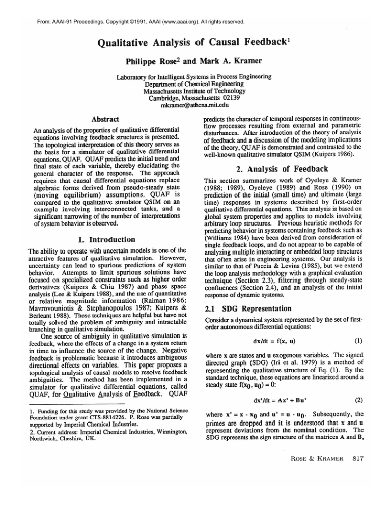
Consider a dynamical system represented by the set of fiistorder autonomous differential equations:
dx/dt = f(x, u)
where x are states and Mexogenous variables. The signed
directed graph (SDG) (Iri et al. 1979) is a method of
representing the qualitative structure of Eq. (1). By the
standard technique, these equations are linearized around a
steady state f(xg, uo) = 0:
dx’/dt = Ax’ + Bu’
1. Funding for this study was provided by the National Science
Foundation under grant CTS-8814226. P. Rose was partially
supported by Imperial Chemical Industries.
2. Current address: Imperial Chemical Industries, Winnington,
Northwich, Cheshire, UK.
(1)
(2)
where x’ = x - x0 and u’ = M - UO. Subsequently, the
primes are dropped and it is understood that x and u
represent deviations from the nominal condition. The
SBG represents the sign structure of the matrices A and B,
ROSE & KRAMER
817
and applies in the domain around (x0, ~0) where
linearization of Eq. (1) yields a constant sign structure for
A and B. The SDG consists of nodes and directed arcs.
Nodes correspond to the system variables x and u, and
have qualitative states (0), (+), and (-), corresponding to xi
(or ui) = 0, xi > 0, and xi c 0, respectively. A directed arc
from xj to xi exists iff Aij # 0. Each NC has an associated
sign + or - corresponding
to Aij > 0 or Aij < 0.
Similarly, an arc from uj to xi represents Bij. The
diagonal elements Aii and Bi are represented as signed self
cycles on nodes. An integrating variable is one with no
self cycle (Aii = 0).
The following SDG structures are defined. A m is a
directed sequence of nodes and arcs in the SDG. An acyclic
& is an open path where all nodes appear only once. A
loop is a closed path (having the same initial and terminal
nodes), where each arc is traversed only once. A cycle is a
loop where each node is traversed only once. Cycles are
said to be Conjunct if they share at least one variable, and
disjunct otherwise. A stronglv connected comDonen[
(SCC) is a maximal subgraph in which a path exists from
any node to any other node. The ComDlementarv
subsystem of a path is the subgraph obtained when all
nodes in the path are removed. The acvclic subsvstem of a
graph is the subgraph obtained when all variables involved
in cycles (excluding self-cycles) are removed.
2.2
Key Results
The initial response of a variable is defined as the first
non-zero sign assumed by a node in response to a
disturbance if the sign of all nodes prior to the perturbation
is (0). The ultimate resDonse of a variable is the final
(steady) state in response to a finite perturbation, under the
assumption that the system remains in the same qualitative
regime, i.e. the SDG is fixed. Transitions between
qualitative regimes, if they occur, are assumed to be
detected and handled by auxiliary procedures.
Local
stability at the initial and final steady states is also
assumed3. Several conclusions concerning the behavior of
systems described by SDGs in response to finite,
monotonic perturbations will now be stated:
1) The initial response of a variable xi to a disturbance ur
is due to the minimum order (shortest) path in the SDG.
Since paths that include loops are never minimum order,
the initial response is the result of disturbance propagation
on minimum order acyclic paths.
2) The ultimate (steady state) response of xi is the sum
of the effects transmitted on acyclic paths if xi is not
contained in a negative feedback loop.
3) If xi is contained in a negative feedback loop, the
ultimate response of the variable is the superposition
3. Criteria for stability of qualitative differential equations are
given by Puccia & Lmins (1985) and Ishida (1989).
818
QUALITATIVE ANALYSIS
(qualitative sum) of the responses to individual inputs of
the SCC containing the variable.
4) If xi represents a variable in an SCC and ur is an
exogenous disturbance to the SCC containing xi, the
ultimate qualitative response of Xi to Ur is:
[Xi] = [ur] 0 [bh(-I)“- ’IPil
(3)
+ 2&i aijbjr(-1)
f &+ij
cj& aijajkbkr(-1)““IPijkl + ...
+ qJ+ ... Zj#i aij...%pbpr(-l)IPijk...pI
f zq# . .. cj#i aik...apqbqrlPijk...pql1
where Pm is the principal minor obtained by deleting the
rows and columns of A corresponding to m, and (-l)“Cl ml represents the signed determinant of that matrix.
The square brackets [=] extract the sign of their argument,
and arithmetic on the qualitative values (+), (-) and (0) is
handled in the usual way.
hical Interpretation
Each product bir, aijbjr, aijajkbkr, etc. in Eq. (3)
represents the net sign of an acyclic path from ur to xi.
The summations cover all possible acyclic paths. The
direct effects of a disturbance on a variable are the
directional influences transmitted on acyclic paths. By
result (l), direct effects account for the initial response. In
the ultimate response, each direct effect is multiplied by
the signed determinant of the matrix obtained by deleting
the nodes of the acyclic path, i.e., the determinant of the
complementary subsystem of the path. The feedback from
the complementary subsystem is termed compensatorv if
the complementary determinant is zero, thus canceling the
direct effect at steady state; overcompensatorv
if the
determinant is negative, reversing the direct effect at steady
state; and JlndercomDensatorv if the determinant is positive,
leaving the direct effect qualitatively unchanged at steady
state.
QUAF applies graphical criteria for determining the
signs of complementary determinants. These criteria were
given in Oyeleye & Kramer (1988), and later refined by
Rose (1990). The criteria are:
a The signed determinant of a graph is zero if and only if
its acyclic subsystem contains at least one integrating
variable, or if the graph contains at least two integrators in
conjunct cycles that are not in the same cycle and not in
disjunct cycles. This case corresponds to compensatory
feedback.
.
The signed determinant of a graph is positive if and
only if it is non-zero by the above criteria, and does not
contain a positive cycle or self-cycle.
This case
corresponds to undercompensatory feedback.
If a graph does not meet either of these criteria, then the
sign of its determinant depends on quantitative attributes.
inal state
2.
Steady state behaviors must be consistent with algebraic
constraints which apply at steady state, i.e. the confluences
formed by setting the time derivatives in the qualitative
differential equations to zero. These confluences, called
nodal balances (since each represents the sum of effects
around an SDG node), admit behaviors that are not
necessarily the same as those produced by analysis of
feedback. Thus, the nodal balances can be used as a filter
for the behaviors predicted by loop analysis.
The nodal balances may remove none, some or all of
the behaviors predicted by loop analysis. If there are no
valid behaviors left after the application of nodal balances,
then there are no steady state behaviors within the
qualitative regime described by the SDG. This means the
disturbance causes the system to exit the qualitative
regime, or possibly to become unstable.
0
The previous results have been translated into an efficient
computer program called QUAF to predict the qualitative
behavior of systems governed by Eq. (1). The following is
a rough procedural outline of QUAF:
1. The SDG is decomposed into a set of strongly
connected components. Information on loops and cycles
is stored for later use.
2. The effect of each perturbation variable is extended to
each affected SCC. For each disturbance variable outside
an SCC, the response of each variable internal to the SCC
is determined by examining each acyclic path from the
disturbance to the SCC variable. The initial response for
each variable is the sign of the disturbance times the net
sign of the shortest acyclic path to the variable.
3. If the SCC variable examined in Step 2 is not located
in a negative loop, the final response to the disturbance is
the qualitative sum of the direct effects. If the variable is
in a negative loop, then:
a. If there is no integrating
variable
in the
complementary subsystem of the acyclic path, go to 3e.
b. If there is an integrating variable in the acyclic
subsystem of the complementary subsystem of
path, the complementary feedback is compensatory. Go to
Step 4.
C.
If there are less than two integrating variables in the
complementary subsystem of the acyclic path, go to 3e.
d If there is a pair of integrating variables in the
complementary subsystem of the acyclic path that are in
conjunct cycles but not in the same cycle and not in
feedback is
disjunct cycles, the complementary
compensatory. Go to Step 4.
e. If the complementary subsystem does not contain a
positive cycle or self-cycle, the complementary feedback
effect is undercompensatory.
Else, the complementary
feedback is possibly overcompensatory.
4. The ultimate response of the SCC variable is
ambiguous if the complementary feedback of any direct
effect is possibly overcompensatory.
Otherwise, the
ultimate response is sum of the direct effects whose
complementary feedback effects are undercompensatory.
The final response is (0) if all direct effects have
compensatory feedback.
5. The final response pattern for each disturbance is
filtered through the steady-state nodal balance constraints.
3.
Algebraic Equations
QUAF requires the system model to be expressed in terms
of qualitative differential equations. Definitional equalities
can be handled as auxiliary equations, but other algebraic
equations must be replaced by differential equations.
QUAF’s prohibition on algebraic equations can be
interpreted as enforcement of causal structure on the model.
Algebraic equations imply instantaneous, non-local
transmission of effects, contrary to the interpretation of
causality as local propagation of effects in a device
(Bobrow
1984). For example, the equation for
incompressible turbulent flow in a pipe, F = k(Pin Pout)l”, is noncausal because a change in inlet pressure
must be accompanied by instantaneous change in outlet
pressure or flow, essentially an effect at a distance. The
algebraic equation reflects the “moving equilibrium”
approximation that equilibration of pressure and flow is
much faster than other changes of interest. While moving
numerical
equilibrium
may be an acceptable
approximation, use of the algebraic form involves loss of
information on device causality.
Although equilibration of pressure and flow is very
rapid, it is not instantaneous. To model action on time
scales below the model granularity, deKleer and Brown
(1984) introduce “mythical causality” and heuristics to
describe change during mythical time. We do not think it
is desirable to introduce special heuristics to account for
behavior on short time scales. Instead, we revert algebraic
equations back to differential form and then analyze them
in the rigorous fashion given above. For example, flowpressure dynamics in a pipe for our purposes are described
as adF/dt = k(Pin - Pout)l/2 - F, where a is a small
parameter related to fluid compressibility. Re-introduction
of causality is based on device physics, not equation
structure, because in feedback structures it is not possible
to recover the causality by the simple expedient of equation
ordering (Iwasaki and Simon 1986). Physical knowledge
of causality in short time scale processes is required to
replace that loss.
e
xample
This section demonstrates the qualitative analysis of
feedback on a system of gravity-flow tanks, shown in Fig.
1. The objective is to simulate the response of the system
to various faults involving leaks and blockages. The state
variables for this system are the levels, pressures and
flows: Ll, PI, Fl, L2, P2, F2, F3, Pjunc, and F4. The
variables AP pump, QL Q2, W-R4 represent system
faults (pump failure, leaks, and blockages).
ROSE & KRAMER
819
dLl/dt=Fo+Fs-Fl-Ql
d.Ll/dt=Fo+Fg-Fl-Q1
PI= M+(Ll)
a dPl/dt = M+(Ll) - P1
F1 = (P1)1’2/h
a dFl/dt = (P#/2/Rl-
dL2/dt=Fl+FyQ2
dLddt=Fl+Fz-Q2
P2 = M+(Lz>
a d.P2/dt = M+&)
F2 = (P2+mpump-Pjunc)
1’2m2
F3 = (Pjunc)1’2B3
F4 = (Pjunc)1’2R4
Fz=Fs+Fq
F1
- P2
a dF2/dt = (P2+hPpump-Pjunc)l/
- F2
a dF3/dt = (Pj&1/2/R3 - F3
a dF4/dt = (Pjunc)‘/2/Rq - F4
a dPjunJdt = F2 - F3 - F4
Table 1. Equations for example. Non-causal form (left) and causal form (right).
4.1
Modeling
Considerations
The model equations, as conventionally written, are given
in the first column of Table 1. This form is not suitable
for qualitative analysis of feedback because of moving
equilibrium assumptions in the pressure-flow expressions.
Rewriting the model in causal form leads to the equations
in the second column of Table 1. The SDG, shown in Fig.
2, is derived from the signs of the partial derivatives in the
causal equations. For example, the first equation becomes
the confluence &] = IFg] + cF3] - PI] - [Ql], represented
by four inputs to the node Ll. L1 is an integrating
variable because it does not influence its own rate of
change. In contrast, F1 has a negative self-cycle because
its differential confluence contains -[Fl] on the right hand
side.
Initially, each variable is assumed have the qualitative
state (0). Fault simulations are conducted by assuming a
change in one of the fault parameters to (+) or (-).
Without qualitative analysis of feedback, this system
displays numerous ambiguous behaviors. For example, if
pipe 1 resistance RI is increased, Fl will initially tend to
decrease; however the subsequent increase in Ll generates
an increased pressure head PI that tends conversely to
increase Fl. If one assumes the negative feedback effect on
FI from Ll can overcome the initial (direct) effect, leading
to Fl(+), then subsequent propagation through the SDG is
capable of predicting almost any variable in any state. The
explosion of ambiguity is characteristic of systems
involving negative feedback.
4.2
Results of Analysis by
The QUAF program determined the initial and final
responses of this system for all seven faults using the
SDG shown in Fig. 2 in approximately one-half second of
820
QUALITATIVE ANALYSIS
CPU time on a DEC-3100 workstation. The results are
given in Table 2. Table 2 lists both the results of the
analysis of feedback, and the final responses after filtering
by steady state nodal balances. A unique final state was
predicted in all but two cases after application of nodal
balances. In all cases, a unique initial state was predicted.
We include the following examples to demonstrate the
procedures involved in the analysis of feedback:
Case 1: Effect of RJ on Fl. There is only one acyclic
path from R1 to F1, and therefore the direct effect is
unambiguous; the initial response to RI(+) is Fl (-) .
Since Fl is contained in a negative feedback loop,
complementary feedback must be considered in the ultimate
response. The complementary subsystem to the acyclic
pati Rl to Fl is (I-+ PI, J-2, P2, FL F3, Pjunc, F4).
There are three integrating variables in the complementary
subsystem: Pjunc, Ll, and L2. The acyclic subsystem of
the complementary subsystem consists of only Ll, an
integrating variable, and therefore the complementary
feedback is compensatory. This guarantees that the final
value of Fl in response to an increase of R1 is (O)(-) = (0).
Therefore, F1 initially decreases but eventually returns to
normal in response to a partial blockage of pipe 1.
Case 2: Effect of mm.
There are two acyclic paths
from R4 to F2, (Rq + F4 + Pjunc + Fz>~which is net
negative, and (R4 + F4 + Pjunc + F3 -+ L1 + P1 +
F1 3 L2 + P2 + F2), which is net positive. The initial
response is determined by the lowest-order path, therefore
the initial response to R4(+) is F2(-). Since Fq is
contained in a negative feedback loop, complementary
feedback is a factor in the ultimate response.
The
complementary subsystem of the first acyclic path is {Ll,
PI, Fl, L2, P2, F3), which contains integrating variables
L1 and L2. The acyclic subsystem of the complementary
F3
-=-I#
FO - F4
Ll,L2
Pl,P2
R3
Pjunc
%-g
Stream flow rates
Tank levels
Discharge pressures
Leakages
Pipe resistances
Pump pressure head
Pressure at junction
F4
APpump
Figure 1. Recycle Tank System
FO
Figure 2. SDG of Recycle Tank System
subsystem is (F3, L2, P2). Since L2 is an integrating
variable, complementary feedback to the first acyclic path
is compensatory. The complementary subsystem of the
second acyclic path is the empty graph. The empty graph
does not contain an integrating variable, nor a positive
self-cycle or loop, so the complementary feedback for the
second acyclic path is undercompensatory. The ultimate
response is therefore (-)(0) + (+)(+) = (+). Thus, F2
initially decreases but then rises above its nominal value in
response to a partial blockage of pipe 4.
arison with Q§IM
QSIM and QUAF are different in design and intention
and should not be viewed as “rival” methods. Some major
differences between QSIM and QUAF are:
0 QSIM states are represented as {value, derivative),
with value given relative to one or more landmarks; in
QUAF the only landmark is the nominal state (0), and the
derivative is not represented.
0 Models in QSIM are QDAEs (qualitative differentialalgebraic equations), while QUAF accepts only QDEs
(qualitative ordinary differential equations).
m A variety of constraint relationships can be specified
in QSIM (additive, multiplicative, derivative, analytic
function, direction of change, etc.), while QUAF deals
only with first-order differential confluences.
a QSIM produces a detailed incremental history for each
variable; QUAF only elucidates the general character of
trajectories based on initial deviations and final states.
0 QSIM provides mechanisms for handling transitions
to other qualitative domains; QUAF assumes the same
qualitative model applies throughout the simulation.
Despite these differences, the number of initial and
ultimate behaviors produced by QSIM and QUAF for the
recycle tank example can be meaningfully compared. The
QSIM model for the tank system was derived from the
equations given in the first column of Table 1.
Transitions between qualitative regimes were inhibited by
the use of the “unreachable-landmark” constraint on the
tank levels, and “chattering” behaviors on tank flows were
inhibited.
For each fault, the number of distinct initial states (in
terms of states, ignoring directions of change) and the
number of quiescent states eventually reached were counted.
In five out of seven cases, QSIM produced multiple initial
and final states, while in five of seven cases QUAF did
not. Table 3 lists the number of interpretations produced
by QSIM and QUAF. The results for QSIM do not
include the total number of distinct variable histories, but
only the number of distinct initial and final states.
The excess behaviors generated by QSIM are spurious,
and any temporal histories inconsistent with QUAF results
could be pruned. Excess behaviors result from the fact that
ROSE & KRAMER
821
Table 2: Analysis of Feedback for Recycle Tank System
I-E VARIABLE
DISTURBANCE
I
I
R3c
Ll, PI
Fl
L2, P2
F2
Pjunc
F4
Dir = +
hit = +
Det=+
Fin I= +
Dir = +
lnit = +
Det=+
Fin = +
Dir = +
lnit = +
Det=+
Fin = +
Dir = +
lnit = +
Da=+
Fin = +
Dir=+
hit = +
Da=+
Fin = +
Dir = +
lnit = +
Det=+
Fin = +
Dir = +
lnit = +
Det=+
Fin = +
Dir = + , hit = +
Det=+,+
Fin = +,O, -
Dir = lnit = Det=o
Fin = 0
Dir = lnit = Det=o
Fin = 0
Dir = hit = Det=o
Fin = 0
Dir = hit = Da-0
Fin = 0
Dir = hit = Det=O
Fin = 0
Dir = lnit = Det=o
Fin = 0
Dir = lnit = Det=+
Fin = -
Dir = lnit = Det=+
Fin = -
Dir = lnit I Det=+
Fin = -
Dir = lnit = Det=+
Fin = -
Dir = hit = Det=+
Fin = -
Dir = lnit = Det=+
Fin = -
Dir = lnit = Det=+
Fin = -
Dir = lnit = Det=o
Fin = 0
Dir = lnit = Det=o
Fin = 0
Dir = +, lnit = +
Det=+,+
Fin = +,O,-
Dir = lnit = Det=O
Fin = 0
Dir = hit = Det=o
Fin = 0
Dir = lnit = Det=O
Fin = 0
Dir = lnit = Det=O
Fin = 0
Dir 5 lnit = Det=+
Fin = -
Dir = lnit = Det=+
Fin = -
Dir = +, lnit = +
oat=+,+
Fin = +,O,-
Dir = -, lnit = Det = 0, +
Fin = -
Dir = +, hit = +
Det = +, +
Fin = +,O,-
Dir = lnit = Det=+
Fin = -
Dir = +, lnit = +
Det = +, +
Fin, = +,O,-
Dir = +
lnit = +
Da=+
Fin = +
Dir = +
lnit = +
Det=+
Fin = +
Dir = +, +
hit = +
Det=+,+
Fin = +
Dir = +, hit = Da=+,0
Fin = +
Dir = +
hit = +
Det=+
Dir = +
lnit = +
Det=+
Fin = +
Dir = lnit = Det = -?
Fin = +,O,-
Dir = Direct effect(s)
lnit = Predicted initial response
Det = Determinant(s) corresponding to direct effects
Fin = +
aFinal response after nodal bal. = {+,O,O,O,O,O,O}
bFinal response after nodal bal. = {O,O,+,O,O,O,O}
Fin=predicted
finalresponse(s)
&foreno&lbalances
’Final
respnses
afier
n0dal
bal*
={-~-I-~-~-~-~-)~
I-,-,-,-,O,-,O} and (-,-,?,-,+,-,+}
QSIM
QUAF
initial final
Table 3. Number of
interpretations by QSIM
and QUAF for recycle
tank system.
822
QUALITATIVE ANALYSIS
initial final
1
3
1
1
1
1
1
1
3
4
1
1
1
1
1
1
3
4
1
1
3
4
1
1
2
5
1
5
1
3
1
3
QSIM propagates change by local rules and does not
consider the global properties of the system in the same
way as QUAF. Thus, qualitative analysis of feedback
could complement the simulation paradigms already
incorporated into QSIM.
Kuipers, B.J. 1986. Qualitative
Simulation. Artificial
Intelligence 29:289-338.
Kuipers, B.J.; and Berleant, D. 1988. Using Incomplete
Quantitative Knowledge in Qualitative Reasoning. Proc.
7th Natl. Conf. on Artificial Intelligence, 324-329.
5. Conclusions
The proposed method for interpreting the behavior of
causal models of dynamic systems is capable of yielding
very focused interpretations of system behavior, even when
there are complicated feedback and control structures. The
method has a rigorous foundation and operates entirely
from qualitative considerations.
Without using this
method to resolve feedback effects, qualitative reasoning
can become muddled in circular chains of cause and effect,
producing a large number of spurious behaviors. This
paper shows that the resolution of feedback effects can be
accomplished
straightforwardly,
without additional
quantitative information, when models are structured
causally.
Acknowledgements
The authors are grateful to Mr. Jack Vinson and Prof. Lyle
Ungar of the Univ. of Pennsylvania for conducting the
QSIM simulations. Dr. 0.0. Oyeleye made valuable
contributions in the early stages of this research.
eferences
Bobrow, D.G. 1984. Qualitative Reasoning About
Physical Systems: An Introduction. Artificial Intelligence,
24: l-5.
De Kleer, J.; and Brown, J.S. 1984. A Qualitative
Physics Based on Confluences. Artificial Intelligence,
24:7-84.
Iri, M.; Aoki, K.; O’Shima, E.; and Matsuyama, H. 1979.
An Algorithm for Diagnosis of System Failures in the
Chemical Process. Comput. Chem. Engng. 3:489-493.
Ishida, Y. 1989. Using Global Properties for Qualitative
Reasoning: A Qualitative System Theory. Proc. 13th Intl.
Joint Conf. on Artificial Intelligence, 1174-l 179.
Iwasaki, Y.; and Simon, H.A. 1986. Causality in Device
Behavior. Artificial Intelligence 29:3-32.
Kuipers, B.J.; and Chiu, C. 1987. Taming Intractable
Branching in Qualitative Simulation. Proc. llth Intl.
Joint Conf. on Artifical Intelligence, 1079-1085.
Lee, W.W.; and Kuipers, B.J. 1988. Non-Intersection of
Trajectories in Qualitative Phase Space: A Global
Constraint for Qualitative Simulation. Proc. 7th Natl.
Conf. on Artificial Intelligence, 286-290.
Mavrovouniotis, M.L.; and Stephanopoulos, G. 1987.
Reasoning with Orders of Magnitude and Approximate
Relations. Proc. 6th Natl. Conf. on Artificial Intelligence,
626-630.
Oyeleye, 0.0. 1989. Qualitative Modeling of Continuous
Chemical Processes and Applications to Fault Diagnosis.
Sc.D. diss., Dept. of Chem. Engng., Massachusetts Inst.
of Tech.
Oyeleye, 0.0.; and Kramer, M.A. 1988. Qualitative
Simulation of Chemical Process Systems: Steady-State
Analysis. AXhE J. 34:1441- 1454.
Oyeleye, 0.0.; and Kramer, M.A. 1989. The Role of
Causal and Noncausal Constraints in Steady-State
Qualitative Modeling.
In Artificial
Intelligence,
Simulation and Modeling, Widman, Loparo, Nielson, eds.
New York: Wiley.
Puccia, C.J., and Levins, R. 1985. Qualitative Modeling
of Complex Systems. Cambridge, Mass.: Harvard Univ.
Press.
Rose, P. 1990. A Model-Based System for Fault
Diagnosis of Chemical Process Plants, MS. diss., Dept.
of Chem. Engng., Massachusetts Inst. of Tech.
Raiman, 0. 1986. Order of Magnitude Reasoning. Proc.
5th Natl. Conf. on Artificial Intelligence, 100-104.
Williams, B.C. 1984. Qualitative Analysis of MOS
Circuits. Artificial Intelligence, 24~281-346.
ROSE AL KRAMER
823
