Learning From Demonstrations via Structured Prediction
Charles Parker, Prasad Tadepalli, Weng-Keen Wong, Thomas Dietterich, and Alan Fern
Oregon State University
School of Electrical Engineering and Computer Science
Corvallis, OR 97333
{parker,tadepall,wong,tgd,afern}@eecs.oregonstate.edu
Abstract
This presents us with a problem, however, when we are
faced with a world state not seen in the demonstration plans.
In this case, the student has no notion of how to proceed
and can do no better than to act randomly. Clever, featurebased representations of the value function allow generalization over the state space, but we are still learning the objective function indirectly. That is, the above approach learns a
value function over the entire state space and then attempts
to maximize the value of constructed path.
As an alternative approach, we propose direct, discriminative learning of this function. Rather than ask the question,
“What is the value of each state in the state space” we will
ask, essentially, “What separates ‘good’ states from ‘bad’
ones?”. Recent work in structured prediction has given us a
framework to do exactly this.
In the next section we describe this work and relate it to
our approach. We later derive our gradient boosting method
and give experimental results in a sub-domain of Wargus,
a real-time strategy game. The results show that our system
learns to plan effectively from a small number of demonstrations even when there are many irrelevant features.
Demonstrations from a teacher are invaluable to any
student trying to learn a given behavior. Used correctly,
demonstrations can speed up both human and machine
learning by orders of magnitude. An important question, then, is how best to extract the knowledge encoded
by the teacher in these demonstrations. In this paper, we
present a method of learning from demonstrations that
leverages some of the structured prediction techniques
currently under investigation in the literature. We report encouraging results in Wargus, a real-time strategy
game.
Introduction
Humans learn to interact with the world in a variety of complex ways. One of these ways is learning by demonstration.
In this paradigm, a “teacher” presents a “student” with a plan
to accomplish a given goal, usually formalized in machine
learning literature as a sequence of actions. The student can
then generalize the world state to which the demonstrated
plan applies to other states where the plan may also apply.
Often, the demonstration plan is one of an exponential
number of plans that may satisfy a given goal set, and in
many domains (such as routing and scheduling), satisfying the goals of planning may be almost trivial. The higher
achievement then, is to find a plan that satisfies the goal set
optimally, or at least much better than the average, randomly
drawn, goal-satisfying plan. Implicit in the above description is the notion that the demonstrated plan is one such “optimal” or “much better than average” plan.
In the reinforcement learning literature, the student typically learns through exploration. The student is allowed to
take random actions in the world, and whenever one of these
actions is taken, a reward is given. Over the course of many
thousands of random actions, it becomes clear to the student
which actions and world states generate the most reward.
The best sequence to accomplish the given goal, then, becomes the sequence of actions that takes the student through
the sequence of world states with the highest reward. In
this setting, learning by demonstration guides exploration by
“showing” the student a number of high-utility states, thus
eliminating the need to discover them by random action.
Related Work
This work is related to three threads of work in machine
learning. One is structured prediction (Taskar 2004), and
particularly the work on cutting-plane methods as seen in
(Tsochantaridis et al. 2004) and in (Parker, Fern, & Tadepalli
2006). In the vocabulary of supervised, multi-class learning,
this work focuses on problems where there are an exponentially large number of negative classes for each training example. The approach is essentially to choose one of the best
misclassifications for each positive example, and to update
the model so that the correct class is chosen over this misclassification. In this way, problems having exponentially
large numbers of classes can be solved efficiently.
The second strand is inverse reinforcement learning (Ng
& Russell 2000). Here we assume that the demonstrated behavior is the result of optimally solving a Markov Decision
Process (MDP). The task is to learn the unknown reward or
cost function of the MDP from the demonstrated trajectories
of its optimal solution. One approach to this problem is to assume that all the other trajectories to be suboptimal and learn
reward functions which maximally distinguish the optimal
trajectories from the suboptimal ones. Since the number of
c 2007, Association for the Advancement of Artificial
Copyright Intelligence (www.aaai.org). All rights reserved.
34
si , with optimal action ai . Specifically, suppose that aˆi ∈ A
is the best non-optimal action given the current weights:
suboptimal solutions is exponential in the size of relevant
parameters, this problem is similar to the structured prediction task and is tackled by a similar iterative constraint generation approach. In each iteration, the MDP is solved optimally for the current reward function, and if the optimal solution generates a trajectory different from the demonstrated
trajectory, it is used to train the next version of the reward
function which maximally separates the optimal trajectories from the suboptimal trajectories (Abbeel & Ng 2004;
Ratliff, Bagnell, & Zinkevich 2006).
The task we study in this paper is more naturally formulated as learning to act from demonstrations (Khardon
1999). Unlike inverse reinforcement learning that tries to
learn the reward function, thus indirectly defining an optimal
policy, here we directly seek to distinguish good state-action
pairs from bad state-action pairs. Each state-action pair is
described by a feature vector, and the optimal state-action
pairs are assumed to maximize a weighted sum of its features. Thus, learning the weights of this optimizing function
is sufficient to generate optimal behavior. Unlike in inverse
reinforcement learning, the weights need not correspond to
reward values. They merely need to distinguish good actions
from bad actions as well as possible.
aˆi = argmax w · Ψ(si , a)
a∈A,a=ai
(1)
Our weights, then, must be engineered so that, for si ,
w · Ψ(si , aˆi ) < w · Ψ(si , ai )
(2)
for all demonstrations {si , ai } ∈ T .
It is possible that there are zero or infinitely many choices
for w that accomplish this goal. We will then attempt to
find a w that minimizes some notion of loss and maximizes
a notion of margin. Our margin at each training example
{si , ai } ∈ T is clearly
w · Ψ(si , ai ) − w · Ψ(s, aˆi )
(3)
We use a margin-based based loss function defined in previous work (Friedman, Hastie, & Tibshirani 2000), log(1 +
exp(−m)), where m is the margin. The cumulative loss L
over the training set is
L=
log[1 + exp(w · Ψ(si , aˆi ) − w · Ψ(si , ai ))] (4)
i
Gradient Boosting for Plan Optimization
Our problem can be formulated as a four-tuple {S, A, T , R},
where S is a set of possible world states, A is a set of possible actions, and R is a reward function such that R : s ∈
S × a ∈ A → gives the reward for taking action a
in state s. T is our training set of demonstrations, composed of pairs of the form {s, a} where s is a world state
and a is the optimal (or near-optimal) action to take given
this state. Our ultimate goal, then, is to build a function f
that chooses the correct action for any given state, so that
f (s) = argmaxa∈A R(s ∈ S, a). To build f , we will rely
on the techniques of structured prediction as stated above. In
particular, we use a gradient boosting technique first used in
(Dietterich, Ashenfelter, & Bulatov 2004) and later applied
to structured prediction in (Parker, Fern, & Tadepalli 2006).
Our approach proceeds as follows: We are given a set
of “demonstrations” that take the world from one state to
another in a way that is optimal or near-optimal. We then
attempt to iteratively learn a parameterized linear function
that correctly discriminates the optimal demonstration action from one drawn at random. In each iteration, we select,
from a group of random actions, the best “alternative” to
each demonstration action given the current function. Based
on the demonstrations and the alternatives (that we hope to
avoid), we compute a gradient at each parameter and take
a step in this direction, ideally away from the alternatives
and toward the demonstrations. Furthermore, the gradient is
margin-based so that demonstrations that are already highly
ranked against their alternatives receive less attention than
ones that are not as highly ranked.
To formalize this, we first define the function Ψ(s, a) extracts a joint feature vector that may depend on s, a, and/or
the state of the world that results from the execution of a in
s. We seek a set of weights w that gives a higher value to the
demonstration action than to all other actions, given the state
If there are n features in Ψ(s, a), and Ψj (s, a) gives the
value of the jth feature, we note that
w · Ψ(s, a) =
n
wj Ψj (s, a)
(5)
j
Define the following notation for convenience:
ΨΔj (si ) = Ψj (si , aˆi ) − Ψj (si , ai )
(6)
Finally, suppose our current cost function is wk . The gradient for the loss expression can be derived at each feature
in the representation as follows:
∂L
∂Ψj (s, a)
ΨΔj (si ) exp(wk · Ψ(si , aˆi ) − wk · Ψ(s, ai ))
=
1 + exp(wk · Ψ(si , aˆi ) − wk · Ψ(s, ai ))
i
ΨΔj (si )
=
1
+
exp(w
ˆi ))
k · Ψ(si , ai ) − wk · Ψ(s, a
i
δk+1 (j) =
The new cost function is then wk+1 = wk −αδk+1 where
α is a step size parameter. We can then choose a new â for
each training example and recompute the gradient to get an
iteratively better estimate of w. Once the iterations are complete, and we have a final weight vector, wf , we have successfully constructed the function f from the problem formulation above:
f (s) = argmaxwf · Ψ(s, a)
a∈A
35
(7)
(a) An example of poor base cohesion.
(b) An example of good base cohesion.
Figure 1: Examples of floor plans in the Wargus domain.
Empirical Evaluation
tower x and zero otherwise. If the battle front of a given
map is composed of squares g1 , . . . , gm , then the defensive quality d of a map with two towers is
m
t1 (gm ) + t2 (gm )
(8)
d = i=1
2m
We perform our experiments in the Wargus floor planning
domain described below. Our general approach is to design
several, not necessarily linear, objective functions in this domain and attempt to learn them using the method described
above. We show that learning a linear function in several
simple features is sufficient to approximate the behavior of
these more complex objectives, even where many of the features given are irrelevant.
• Base Cohesion: It is beneficial to locate buildings close
to one another. This makes the base easier to defend
from attack. Formally, if the locations of the buildings are
b1 , . . . , b4 then the cohesion quality c is computed as
4 4
i=1
j=i+1 2n − ||bi − bj ||1
.
(9)
c=
12n
The factor 2n is the maximum distance possible between
any two entities on the map.
• Resource Gathering: The lumber mill should be located
to minimize the average distance between itself and the
various forested areas, and the town hall should be located
as closely as possible to the mine. Formally, suppose the
town hall is at t, the gold mine at m, the lumber mill at
l, and the four forested areas at a1 , . . . , a4 . The resource
gathering quality r of the base is then:
The Wargus Floor Planning Domain
Wargus is a real-time strategy game simulating medieval
warfare. A subproblem in Wargus is the planning of a military base whereby the layout of the buildings maximizes
certain quantitative objectives. In general, the goals are to
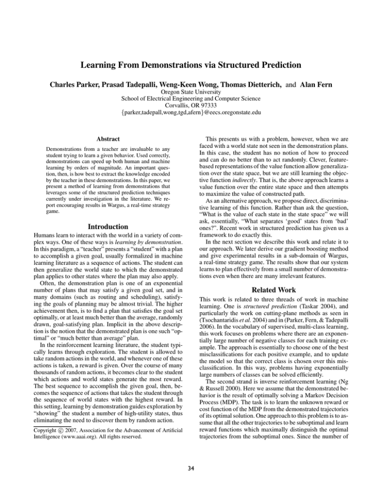
maximize the influx of resources and to survive any incoming attack. Figure 1 shows some examples.
More specifically, we consider a simplified version of
Wargus in which there are two types of natural features on
the map, which is an n × n grid. The first is a gold mine,
and the second is a forested area. On each generated map,
there is one randomly placed mine and four randomly placed
forested areas. Our goal is to place four buildings on the
map so that our objective quantities given below are optimized. These buildings are a town hall, a lumber mill, and
two guard towers. The town hall is a storage building for
mined gold. The lumber mill serves the same function for
cut lumber. The towers are able to fire cannon in a given
radius, providing defenses for the base.
We postulate three such quantitative objectives based on
user experience. For a given map and placement of buildings, we calculate a number between zero and one as a measure of how well each of these goals are satisfied.
4
r=
i=1
2n−||l−ai ||1
8n
2
+
2n−||t−g||1
2n
(10)
Domain Specifics
First note that in this domain, an entire plan, from start to finish, consists of a single, factored action (the placement of all
buildings). Thus, we are in a special case of general MDPs
which allows us to unify reward function and discriminant
action-value function. However, our approach directly applies to general MDPs where we can design a feature space
that allows a linear discriminant function to nearly optimal
and suboptimal actions in any relevant states.
Our experiments are done on a 10 × 10 grid. Thus, there
are tens of millions of possible plans to consider for a given
map. To generate a negative example for each iteration of
• Defensive Structure: In the case where there is a clear
part of the map from which an attack might originate, as
much of this area as possible should be covered by the
attack area of the guard towers. Formally, suppose that
tx (g) returns 1 if grid square g within the attack radius of
36
0.85
0.85
0.8
0.8
0.75
Solution Quality
Solution Quality
0.75
0.7
0.65
0.6
0.55
0.55
0.45
0.4
0.5
0
5
10
15
Iteration
20
25
30
0
(a) α = 0.33, β = 0.33, γ = 0.33
0.9
1
0.85
0.9
0.8
0.8
Solution Quality
0.7
0.65
0.6
Boosted Model
Optimal Model
Random Model
0.55
5
10
15
Iteration
20
25
30
(b) α = 0, β = 0.5, γ = 0.5
0.75
Solution Quality
Boosted Model
Optimal Model
Random Model
0.65
0.6
Boosted Model
Optimal Model
Random Model
0.5
0.7
0.7
0.6
0.4
0.5
0.3
0.45
0.2
0.4
Boosted Model
Optimal Model
Random Model
0.5
0.1
0
5
10
15
Iteration
20
25
30
0
(c) α = 0.5, β = 0, γ = 0.5
5
10
15
Iteration
20
25
30
(d) α = 1, β = 0, γ = 0
Figure 2: Boosting curves for two objective functions in the Wargus floor planning domain. The training set contains 15 maps.
the algorithm (the aˆi of Equation 2), we generate 10000
random plans and choose the best one according to the current model. The plans are pre-screened so that they are valid
placements (i.e., so that multiple buildings are not located
on the same grid square).
Experimental Results
In Figure 2 we see the results of boosting a random model
for 30 iterations according to our algorithm. We evaluate
the model at each iteration on 20 different random maps by
choosing for each map, according to the model, the best in
a random sample of 10000 plans. The chosen plans are then
evaluated according to the optimal model. As the iterations
of the algorithm progress along the horizontal axis, the quality of the plan chosen by the model increases, as expected.
For reference, we plot the performance of the optimal
model as well as the performance of a linear model with its
weights randomly initialized, evaluated in the same way as
the boosted model. Note that the score of the optimal model
varies due to the fact that first, the optimal score of a map
varies from map to map, and second, the optimal plan may
not be in the random sample. As can be seen from the plots
in Figure 2, however, much of this variability is removed as
our experiments are repeated and averaged over ten trials.
We first note that, in every case, the boosted function is
able to learn a floor planning algorithm that is closer to optimal than random. This is true in particular for Figure 2(b),
where the performance of the model converges to performance extremely close to the optimal. This is because the
cohesion and resource gathering quality measures are almost
Given this, note that it is impossible to receive a perfect
quality score of one on all of these measures. For example,
to achieve perfect quality on the resource gathering measure,
the lumber mill would have to be located on the same grid
square as all of the forested areas, which would also have to
be located on the same grid square.
The features in the model are of two types. First, there is
a feature for the Manhattan distance between each building
and each other entity on the map, resulting in 4 × 9 = 36
features. We also give features for the distance from each
building on the map to the closest battle front square, which
results in four more features, for a total of 40 features. Note
that many of these features (the distance from either tower to
any of the forested areas, for example) are irrelevant to plan
quality.
To generate several objective functions in this domain, we
compute the total quality q = αd + βc + γr. We then vary
α, β, and γ to obtain a variety of functions.
37
0.85
0.85
0.8
0.8
0.75
0.65
Solution Quality
Solution Quality
0.75
0.7
Boosted Model
Optimal Model
Random Model
0.6
0.55
0.7
0.65
Boosted Model
Optimal Model
Random Model
0.6
0.5
0.55
0.45
0.4
0.5
0
2
4
6
8
10
12
Training Examples
14
16
18
20
0
(a) α = 0.33, β = 0.33, γ = 0.33
2
4
6
8
10
12
Training Examples
14
16
18
20
(b) α = 0, β = 0.5, γ = 0.5
Figure 3: Learning curves for two objective functions in the Wargus floor planning domain.
room for improvement in the inference portion of the algorithm. As stated before, a best plan is chosen by drawing
randomly from the space of possible plans and choosing the
best one. This is both highly inefficient and unreliable: Depending on the domain, we may have to evaluate thousands
or millions of plans before coming across a reasonable one,
and even then there is no guarantee of quality. This not only
makes inference unreliable, but has a detrimental effect on
learning, as the inference algorithm rebuilds the training set
at each iteration. A better inference routine may improve the
quality of learning and will certainly make it more efficient.
Finally, it is possible that other methods of structured prediction can be specialized for learning via demonstration.
Given the close relationship of gradient boosting (Parker,
Fern, & Tadepalli 2006) to SVM-Struct (Tsochantaridis et
al. 2004), we feel that SVM-Struct is a likely candidate.
directly expressible as linear functions of the given features.
The defense measure is not readily expressible as a linear
function. However, we see in Figure 2(d) that we are even
able to learn a reasonable model when the defense measure
is the only component of the objective. Finally, in 2(a), we
see that that model performs admirably when it is forced
to trade off all of the various components of the objective
against one another.
Figure 3 shows learning curves for two of the objective functions from Figure 2. The number of training maps
is plotted along the horizontal axis. Again, as expected,
more training examples improves performance. We see that,
again, we are able to learn more quickly when the defense
measure is removed from the objective. More important to
note, however, is the scale of the horizontal axis. For both
objective functions, we are able to learn good models with
only 10 to 15 training traces, even in the presence of many
irrelevant features.
Acknowledgments
The authors gratefully acknowledge the Defense Advanced
Research Projects Agency under DARPA contract FA865006-C-7605 and the support of the National Science Foundation under grant IIS-0329278.
Conclusion and Future Work
We have presented here a method for learning via demonstration that leverages the structured prediction techniques
currently under investigation in the literature. We use these
techniques to discriminatively learn the best action to perform in a given world state even when there are an exponential number of states and actions. We have demonstrated the
effectiveness of this techniques in the Wargus floor planning
domain. Specifically, we have shown that this approach is
able to learn to satisfy a variety of objective functions with
only a small number training examples, even in the presence
of irrelevant features.
An important future challenge is to relate this work to
other discriminative reinforcement learning techniques such
as inverse reinforcement learning (Ng & Russell 2000) and
max-margin planning (Ratliff, Bagnell, & Zinkevich 2006).
We suspect that these three approaches have a great deal in
common mathematically, and we would like to establish exactly what these similarities are.
Turning to the particulars of our work, there is certainly
References
Abbeel, P., and Ng, A. Y. 2004. Apprenticeship learning via inverse reinforcement learning. In ICML ’04: Proceedings of the 21st International Conference on Machine
Learning, 1. New York, NY, USA: ACM Press.
Dietterich, T. G.; Ashenfelter, A.; and Bulatov, Y. 2004.
Training conditional random fields via gradient tree boosting. In International Conference on Machine Learning.
Friedman, J.; Hastie, T.; and Tibshirani, R. 2000. Additive
logistic regression: a statistical view of boosting. Annals of
Statistics 28(2):337–407.
Khardon, R. 1999. Learning action strategies for planning
domains. Artificial Intelligence 113(1-2):125–148.
Ng, A. Y., and Russell, S. 2000. Algorithms for inverse
reinforcement learning. In ICML ’OO: Proceedings of the
38
17th International Conference on Machine Learning, 663–
670.
Parker, C.; Fern, A.; and Tadepalli, P. 2006. Gradient
boosting for sequence alignment. In AAAI ’06: Proceedings of the 21st National Conference on Artificial Intelligence (AAAI-06).
Ratliff, N. D.; Bagnell, J. A.; and Zinkevich, M. A. 2006.
Maximum margin planning. In ICML ’06: Proceedings of
the 23rd International Conference on Machine Learning,
729–736.
Taskar, B. 2004. Learning Structured Prediction Models:
A Large Margin Approach. Ph.D. Dissertation, Stanford
University.
Tsochantaridis, I.; Hofmann, T.; Joachims, T.; and Altun,
Y. 2004. Support vector machine learning for interdependent and structured output spaces. In Proc. 21st International Conference on Machine Learning.
39