From: AAAI Technical Report WS-00-06. Compilation copyright © 2000, AAAI (www.aaai.org). All rights reserved.
Efficient
Jesus
Gonzalez,
Mining of Graph-Based Data
Istvan
Jonyer,
Lawrence
B. Holder
and
University of Texas at Arlington
Department of Computer Science and Engineering
Box 19015, Arlington, TX 76019-0015
{gonzalez, jonyer, holder, cook}@cse.uta.edu
Abstract
With the increasing amountof structural data being
collected, there arises a needto efficiently mineinformation from this type of data. The goal of this research is to provide a system that performs data mining on structural data represented as a labeled graph.
Wedemonstrate how the graph-based discovery system
Subduecan be used to perform structural pattern discovery and structural hierarchical clustering on graph
data.
Introduction
The amount of data being generated and collected today is quickly overwhelmingresearchers’ abilities to interpret the data. In response to this problem, a number
of researchers have developed techniques for discovering
concepts in databases. Although muchof the collected
data has an explicit or implicit structural component
(e.g., spatial or temporal), few discovery systems are
designed to handle this type of data.
In this paper we demonstrate how a structural discovery system, Subdue, can be used to perform efficient
mining on structural data. The discovery algorithm implemented in this system is used to perform two types
of mining on graph-based data. First, we describe a
method of discovering patterns from examples embedded in graph data. Second, we introduce a method
of performing hierarchical clustering on structural data
using this graph-based discovery system.
Subdue
Subdue (Cook & Holder 2000) is a tool that discovers
patterns embeddedin labeled graphs. Subdue searches
through the space of possible substructure (subgraph)
patterns, evaluating each possible substructure pattern
based on how well it compresses the input graph in
terms of description length.
Once a substructure is discovered, the substructure
is used to simplify the data by replacing instances of
the substructure with a pointer to the newly discovered substructure. The discovered substructures allow
Copyright(~) 2000, AmericanAssociation for Artificial Intelligence (www.aaai.org).All rights reserved.
21
Diane
J.
Cook
abstraction over detail in the original data. Iteration
of the substructure discovery and replacement process
constructs a hierarchical description of the structural
data in terms of the discovered substructures.
Subduerepresents structural data as a labeled graph.
Objects in the data map to vertices or small subgraphs
in the graph, and relationships between objects mapto
directed or undirected edges in the graph. This graphical representation serves as input to the substructure
discovery system. Subdue has been used to discover patterns in domains such as CADcircuit analysis,
chemical compoundanalysis, and scene analysis. Userdefined limits on the number of reported patterns and
on the graph match constrain the algorithm to be polynomial in the size of the input graph (Cook, Holder,
Djoko 1996).
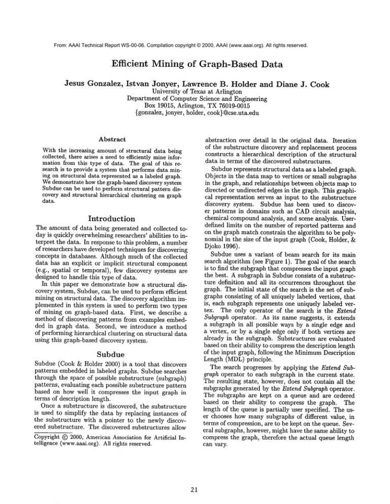
Subdue uses a variant of beam search for its main
search algorithm (see Figure 1). The goal of the search
is to find the subgraph that compresses the input graph
the best. A subgraph in Subdueconsists of a substructure definition and all its occurrences throughout the
graph. The initial state of the search is the set of subgraphs consisting of all uniquely labeled vertices, that
is, each subgraph represents one uniquely labeled vertex. The only operator of the search is the Extend
Subgraph operator. As its name suggests, it extends
a subgraph in all possible ways by a single edge and
a vertex, or by a single edge only if both vertices are
already in the subgraph. Substructures are evaluated
based on their ability to compressthe description length
of the input graph, following the MinimumDescription
Length (MDL)principle.
The search progresses by applying the Extend Subgraph operator to each subgraph in the current state.
The resulting state, however, does not contain all the
subgraphs generated by the Extend Subgraph operator.
The subgraphs are kept on a queue and are ordered
based on their ability to compress the graph. The
length of the queue is partially user specified. The user chooses how many subgraphs of different value, in
terms of compression, are to be kept on the queue. Several subgraphs, however, might have the same ability to
compress the graph, therefore the actual queue length
can vary.
a substructure definition. If the cost of transforming
the instance to become isomorphic to the substructure
definition is less than a user-defined threshold (in the
range [0...1]) multiplied by the size of the larger graph,
the subgraph is considered as an instance of the substructure.
Because the goal of this research is to apply the
substructure discovery algorithm to large, complex
databases, the algorithm is constrained by the values
of Beam and Limit to run in polynomial time. Parallel and distributed versions of the system have also
been developed to provide further scalability (Cook et
al. 2000). The distributed algorithm partitions the
graph into as many subgraphs as available processors.
Each processor searches for subgraphs that compress
the local graph well. After broadcasting the best local substructures to all processors and collecting values based on compressing the description length of all
graph partitions, the best global substructures axe determined. Processors locally expand substructures that
are selected to be amongthe best globally.
Subdue (graph G, int Beam, int Limit)
queue Q = {v [ v has a unique label in G}
bestSub = first substructure in Q
repeat
newQ-- {)
for each S in Q
newSubs = S extended by an adjacent edge
from G in all possible ways
newQ = newQ tJ newSubs
Limit -- Limit - 1
evaluate substructures in newQby compression
of G
Q = substructures
in newQ with top Beam
compression scores
if best substructure in Q better than bestSub
then bestSub = best substructure in Q
until Q is empty or Limit ~ 0
return bestSub
Figure 1: Subdue’s discovery algorithm.
Structural
The search terminates upon reaching a user specified
limit on the number of substructures extended, or upon
exhaustion of the search space. Once the search terminates and returns the list of best subgraphs, the graph
can be actually compressed using the best subgraph.
The compression procedure replaces all instances of the
subgraph in the input graph by a single vertex, which
represents the subgraph. Incoming and outgoing edges
to and from the replaced subgraph will point to, or originate in the new vertex that represents the subgraph.
The Subdue algorithm can be called again on this compressed graph. This procedure can be repeated a userspecified numberof times, and is referred to as an iteration. The maximumnumber of iterations that can be
performed on a graph cannot be predetermined; however, a graph that has been compressed into a single
vertex cannot be compressed further.
Subdue’s search is guided by the MinimumDescription Length (MDL)principle, originally developed
Rissanen (Rissanen 1989). According to this evaluation
heuristic, the best substructure is the one that minimizes the description length of the graph when compressed by the substructure. This compression is calculated as follows:
Compression
Discovery in Earthquake
Data
In this study, we demonstrate Subdue’s ability to
discovery structural patterns in earthquake activity
databases. The earthquake data we analyze contains information from several catalogs (wwwneic.cr.usgs.gov).
provided by sources like the National Geophysical Data
Center of the National Oceanic and Atmospheric Administration. The database has records of earthquakes
from 2000 B. C. to present data. An earthquake record
consists of 35 fields: source catalog, date, time, latitude, longitude, magnitude, intensity and seismic related information such as cultural effects, isoseismal map,
geographic region and stations used for the computations. In this experiment we analyze data covering one
year.
In the graph representation of the data, we used two types of edges to connect the events (earthquakes).
The first type of edge is the "near_in_distance" edge,
which is defined between two events whose distance is
at most 75 kilometers. The second type of edge is the
"nearin_time" edge that is defined between two events
occurring within 36 hours of each other. These parameters were suggested by a professor in the UTAGeology
department, Dr. Burke Burkart. An earthquake event
in graph form is shown in Figure 2.
= DL(S) + DL(G )
DL(G)
Earthquake Data Discovery
where DL(G) is the description length of the input
graph, DL(S) is the description length of the subgraph,
and DL(G] S) is the description length of the input
graph compressed by the subgraph. The search algorithm is looking to maximize the Value of the subgraph
which is simply the inverse of the Compression.
Because variations in the data exist, Subdue employs
an inexact graph match when finding the instances of
Results
Our first sampling of data consisted of 10,135 events,
comprising a graph with 136,077 vertices and 883,358
edges. The first several discovered substructures linked
events with near_in_time and near_in_distance edges.
The fourth discovered substructure is more complex
and is shown in Figure 3. This substructure is interesting because several earthquakes happened in a short
period of time and could be related to a fault placement.
22
Magnitude~
Figure 4: Area of study of Orizaba Fault.
~
Figure 2: Earthquake graph representation.
Substructure
1,19instances
Near_in_time
QNear-in-time
S~
tl
Substructure
2, 8instances
Figure 5: Discovered substructure.
_l~Near-in-time
G
Near_in_time
caused by the Pacific plate, which effects depth based
on the closeness to the Pacific Ocean), then there is
morepossibility that it is related to the fault. However,
we first have to evaluate and determine the depth of
earthquakes caused by subduction in that zone.
In this study we demonstrate that Subdue can be
used to discover patterns in structural data containing
spatio-temporal relations. In this next section we will
describe a different use of the Subduesystem, to perform structural hierarchical clustering.
Near in time
Figure 3: Substructure discovered in earthquake data.
From the discovered results, it was also possible to
conclude from the data that most earthquakes occurred
in the months of May and June and that a frequent
depth for the related earthquakes was 33km and 10km. These depths are validated as frequent depths for
earthquake activity. In next experiment, we use Subdue
to determine the earthquake activity of a specific area
of Mexico. Dr. Burke Burkart, a Geologist at UTA,
has extensively studied the Orizaba Fault in Mexico
(Burkart 1994; Burkart & Self 1985), whose location
shown in Figure 4.
In processing this data, Subduediscovered not only a
subarea with a high concentration of earthquakes, but
also someof the area’s characteristics. The first few discovered substructures indicate that region 59, located
in the state of Guerrero, has the greatest concentration
of earthquakes and that spatial relationships do exist
between earthquakes in this region. Dr. Burkart identified this area as very active.
Figure 5 shows substructures discovered using two
iterations of Subdue. The second substructure, which
is defined in terms of the first substructure, represents
a pattern of some of the events at a depth of 33 Km.
This is a very interesting pattern, because it might give
us information about the cause of those earthquakes.
If the earthquake is not caused by subduction (a force
Hierarchical
Clustering
Using Subdue
Clustering techniques provide a useful means of gaining
better understanding of the data, in manycases through
revealing hierarchical topologies. Clustering has been
applied in diverse fields such as analytical chemistry,
geology, biology, zoology and archeology, and is a key
component in model fitting, hypothesis generation and
testing, data exploration and data reduction. A simple
exampleof hierarchical clustering is the classification of
vehicles into groups such as cars, trucks, motorcycles,
tricycles, and so on, which are then further subdivided
into smaller and smaller groups based on some other
traits.
Current clustering techniques have someintrinsic disadvantages. Statistical and syntactic approaches have
trouble expressing structural information, and neural
approaches are greatly limited in representing semantic
information (Schalkoff 1992). Despite these limitations, a number of clustering algorithms have demonstrated success including Cobweb(Fisher 1987), Labyrinth
(Thompson & Langley 1991), and AutoClass (Cheeseman & Stutz 1996). Hierarchical approaches to cluster-
23
Figure 6: Artificial
domain.
ing including agglomerative methods that merge clusters until an optimal separation of clusters is achieved,
and divisive approaches that split existing clusters until an optimal clustering is found. These approaches
usually have the disadvantage of being applicable only to metric data, which excludes discrete-valued and
structured databases (Guha, Rastogi, & Shim 1998;
Krypis, Han, & Kumar 1999).
Our Graph-Based Hierarchical Conceptual Clustering algorithm uses Subdueto construct the hierarchical
lattice of clusters. The discovered substructure after a
single iteration comprises a cluster. The identified cluster is inserted into the classification lattice and used
to compress the input graph. The compressed graph is
passed again to Subdue to find another substructure.
This iteration allows Subdue to find new substructures
defined in terms of previously discovered substructures.
Previous work suggested the user of classification
trees; however,in structured domainsa strict tree is inadequate. In these domains a lattice-like structure may
emerge instead of a tree. Whensubstructures are added
to the lattice, their parents may include other, nonroot nodes in the lattice. If a substructure is composed
of two of the same previously-discovered substructures,
then there will be two links from the parent to the child
in the lattice.
Subduesearches the hypothesis space of all classification lattices. During each iteration of the search process, numerous local minima are encountered, where the
global minimumtends to be one of the first few minima. For clustering purposes the first local minimum
is used as the best partial hypothesis. The reason for
this is easy to see. Subduestarts with all the singlevertex instances of all unique substructures, and iteratively expands the best ones by a single vertex. The
local minimumencountered first is therefore caused by
a smaller substructure with more instances than the
next local minimum, which must be larger, and have
fewer instances. A smaller substructure is more general
than a larger one, and should represent a parent node
in the classification lattice for any morespecific clusters. Even though it is entirely possible to use the global
minimumas the best substructure, we found that if the
global minimumis not the first local minimumit may
produce overlapping clusters.
To provide an example of the explanation above, the
Figure 7: Classification lattice for artificial
domain.
generation of the hierarchical conceptual clustering for
the artificial domain(shown in Figure 6) is demonstrated here. The resulting classification lattice is shownin
Figure 7.
Subduein the first iteration discovers the substructure that describes the pentagon pattern in the input
graph. This comprises the first cluster, Cp. This cluster
is inserted as a child for the root node. In iterations 2
and 3, the square shape (cluster C8) and the triangle
shape (cluster Ct) are discovered, respectively. These
are inserted at the root as well, since Cs does not contain Cp in its definition, Ct does not contain either Cp
or Vs.
All of the basic shapes (pentagon, square and triangle) appear four times in the input graph. So why is
it than that they are discovered in the order described
above? Since all of them have the same number of instances in the graph, the size of the subgraph will decide
how much they are capable of compressing the input
graph. The subgraph describing the pentagon has five
vertices and five edges, that of the square has four vertices and four edges, and that of the triangle has three
vertices and three edges. Given the same number of
instances, the bigger subgraph will compress the input
graph better.
In the fourth iteration,
Subdue deems the subgraph
the best that describes two pentagon shapes connected
by a single edge. There are two of these formations
in the graph, not four, as one might think, since no
overlapping of instances are permitted. This cluster
is inserted into the classification lattice as the child of
the cluster describing the pentagon, since that cluster
appears in its definition. There are two links connecting
this new cluster to its parent. This is because the parent
cluster definition appears twice.
During iteration five, a subgraph is discovered that
contains a pair of squares connected by an edge, a pair
of triangles connected by an edge, and these two pair
are connected by a single edge. This subgraph has two
instances in the input graph. This cluster is inserted as
a child for two clusters in the first level of the lattice,
which appear in the definition of this new cluster. The
new lattice is depicted in Figure 7. Since both parent
cluster definitions appear twice in the new cluster, there
are two links from each of those parents to the new
node.
by the number of transformations required to transform
the smaller cluster instance into the larger one.
The computation of the quality of a hierarchical clustering is recursive, as expressed by the formula. Because
of this recursive nature of the calculation, the quality of
the root node of the classification lattice is the quality
of the entire clustering.
To computethe quality of a single cluster, all of its
child clusters are pairwise compared and normalized. A
pairwise comparison between child clusters is performed
by comparingeach instance of the larger cluster to each
instance of the smaller cluster using the inexact graph
matching algorithm. The value returned by the inexact
graph matching is an integer signifying the number of
transformations required to transform one graph into
the other. This value is normalized between 0 and 1 by
dividing it by the size of the larger graph. The dissimilarity between any two graphs is never greater than the
size of the larger graph. In addition, each cluster inherits the quality of its children which are simply added to
the total quality.
As suggested by the pairwise comparison of child
clusters, this metric measures the dissimilarity of child
clusters of a cluster. A larger numbersignifies a better
quality.
This evaluation heuristic rewards the desirable properties of hierarchical clusters. Big clusters are rewarded,
since two big disjoint clusters need more transformations to transform one cluster into the other. This is
in spite of the normalization, since two 5-vertex and
5-edge clusters having 1 vertex in commonare 90%different, while two 2-vertex and 1-edge clusters having
one vertex in commonare only 66%different.
Disjoint clusters are also rewarded. The less overlap
two clusters have, the more distant they are according
to the fuzzy matching algorithm, therefore contributing
more into the sum of the normalized distances. A small
number of clusters is rewarded by taking the average
of the comparisons of all the instances, this way offsetting the summingeffect, which would normally reward
a large numberof clusters. As we can see, this evaluation heuristic achieves all of our goals set forth for a
hierarchical clustering metric.
Evaluation
Metrics
Conventional (non-hierarchical) clusterings have been
evaluated by the observation which says that instances
within a cluster should be similar to each other, and
instances in adjacent clusters should be significantly different. The measure suggested by this observation is
InterCluster Distance
IntraCluster Distance ’
where InterClusterDistance is the average dissimilarity between members of different clusters, and
IntraClusterDistance is the average dissimilarity between membersof the same cluster. The larger the clustering quality, the more distinctly defined the clusters,
hence the better the clustering.
In hierarchical clusterings the previously mentioned
metric cannot be applied. The main reason for this is
that clusters are organized into a hierarchy, and are not
completely disjoint. Therefore it does not make sense to
compareall of the clusters to all other clusters to compute the average inter-cluster distance. Instead, only
clusters that have a commonparent may be meaningfully compared.
To develop a good metric for hierarchical conceptual
clusterings, first we need to define what characteristics such clusterings should have. One of the things we
would like to have is the best coverage by the smallest number of clusters possible. This would imply that
clusters are general enough to describe the data while
still defining concepts well. In other words, larger clusters provide better generality.
Another desirable property is big cluster descriptions. The more features a cluster has the more its inferential power (Lebowitz 1987). The tradeoff to this is,
of course, less coverage. A third thing we would like a
clustering to have is minimal or no overlap between its
clusters. No overlap indicates disjoint concepts. Clearly
defined concepts are of primary importance in conceptual clustering.
The above mentioned points can be
applied recursively to all clusters of a classification hierarchy. Therefore quality of the root cluster of the
hierarchy equals to the quality of the entire hierarchy.
According to our new metric, evaluation of the quality of the clustering C (CQc) is computed by the equation shown in Figure 8. In this equation, c represents
the numberof child clusters of C, Hi represents the ith
child of cluster C, Hi,k represents the kth instance of
the ith child of cluster C, I Hi I represents the numberof
instances of the child cluster Hi, and I I Hi II represents
the size of the child cluster definition (numberof edges
plus the number of vertices). The distance(Hi,k, Hi,z)
operation in the numerator is the difference between
the two instances of the two child clusters as measured
ClusteringQuality
=
Experimental
Results
In our first experiment, we comparethe lattice generated by Subdue with the classification
tree produced by
Cobwebon an animal database (Fisher 1987). The data
used for the experiment is given in Table. The animal
data is represented in Subdue as a graph, where attribute names (like Nameand BodyCover) are mapped
to labeled edges, and attribute values (like mammaland
hair) are mappedto labeled vertices. The hierarchical
clustering generated by Cobwebis shown in Figure 9.
Using this unstructured data, both systems generated similar hierarchies. The lattice generated by Subdue
is shownin Figure 10. Using the evaluation measure introduced in the previous section, the clustering generated by Subdue has a quality of 2.6. The classification
25
CQc
/=1
Figure 8: Newmetric for evaluating hierarchical clusters.
mammal/bird
mammal
reptile
bird
fish
amphibian
Figure9: Hierarchicalclustering over animaldescriptions by Cobweb.
BodyTemp:
regulated
Fertilization:
intemal
Name:
bird
Name:
reptile
BodyCover:
comified-skin
Fertilization:
intemat
HeartChamber
three
BodyCover:
scales
HeartChamber
two
Figure 10: Hierarchical clustering over animal descriptions by Subdue.
26
Body Cover
hair
feathres
cornified-skin
moist-skin
scales
Name
mammel
bird
reptile
amphibian
fish
Heart Chamber
four
four
imperfect-four
three
two
Body Temp
regulated
regulated
unregulated
unregulated
unregulated
Fertilization
internal
internal
internal
external
external
Table 1: Animal descriptions.
o
\
CH
o
ongoingefforts are focusing on other structural databases such as molecular biology data and chemical compound data. In addition, we detail methods of using Subdueto generate structural hierarchical clusters.
This algorithm has been demonstrated on animal description data and DNAmolecule data. By using the
graph-based discovery and mining techniques found in
Subdue, structural information can be learned and utilized for a variety of domainsand discovery tasks.
o
O ~ P--OH
H
\
oJ
k
o/
HO ~ ~O
O
\
v
CH~o
~--H--O.
o"
%
CH2 0
b¢,o4
c~
s
s
0
o
%%
I
H
References
k
HO -- P=O
A/
/ ~’~ ~o--~-~
o=P--oM
!
./-~
O = P--OH
"%
A
Burkart, B., and Self, S. 1985. Extension annotation
of crustal blocks in northern central american and its
effect upon the volcanic arc. Geology 13:2226.
Burkart, B. 1994. Geologyof northern central america.
In Donovan, S., ed., Geology o/the Caribean. Jamaican
Geological Society. 265-284.
Cheeseman, P., and Stutz, J. 1996. Bayesian classification (AutoClass): Theory and results. In Fayyad,
U. M.; Piatetsky-Shapiro,
G.; Smyth, P.; and Uthurusamy, R., eds., Advances in Knowledge Discovery
and Data Mining. MIT Press. chapter 6, 153-180.
Cook, D. J., and Holder, L. B. 2000. Graph-based
data mining. IEEE Intelligent Systems 15(2):32-41.
Cook, D. J.; Holder, L. B.; Galal, G.; and Maglothin,
R. 2000. Approaches to parallel graph-based knowledge discovery, to appear in Journal of Parallel and
Distributed Computing.
Cook, D. J.; Holder, L. B.; and Djoko, S. 1996. Scalable discovery of informative structural concepts using
domain knowledge. IEEE Expert 11(5).
Fisher, D. 1987. Knowledgeacquisition via incremental conceptual clustering. Machine Learning 2:139172.
Guha, S.; Rastogi, R.; and Shim, K. 1998. Cure: An
efficient clustering algorithm for large databases. In
Proceedings of the ACMSIGMODInternational
Conference on Managementof Data.
Krypis, G.; Han, E.; and Kumar, V. 1999. Chameleon:
Hierarchical clustering using dynamic modeling. Computer 68-75.
Lebowitz, M. 1987. Incremental concept formation:
UNIMEM.Machine Learning 2(2).
Rissanen, J. 1989. Stochastic Complexity in Statistical
Inquiry. World Scientific Publishing Company.
d
\o
k
HO -- ~O
d
Figure 11: Portion of a DNAmolecule.
tree generated by Cobweb, however, yields a value of
1.74.
To illustrate the clusters that Subdue generates for
structured data, we apply the algorithm to a portion of
a DNAdata shown in Figure 11. In the input graph,
vertices represent atoms and small molecules, and edges
represent bonds. A portion of the classification lattice
generated by Subdue is shown in Figure 12. As the
figure shows, the first level of the lattice represents small
commonly-occurring substructures (covering 61%of the
data). Subsequently identified clusters are based on
these smaller clusters that are combinedwith each other
or with other atoms or molecules to form a new cluster.
Conclusions
The increasing
structural
component of current
databases requires efficient methods for mining structural data. In this paper, we described a graph-based
discovery system called Subdue that is capable of mining structural data stored as a labeled graph.
The experiments presented in this paper demonstrate
that Subdue can discover interesting and repetitive
structural patterns in data. These results were described based on spatio-temporal earthquake data, and
27
C--C
Figure 12: Hierarchical clustering of a DNAmolecule.
Schalkoff, R. 1992. Pattern Recognition. Wiley &
Sons.
Thompson, K., and Langley, P. 1991. Concept formation in structured domains. In Fisher, D. H., and
Pazzani, M., eds., Concept Formation: Knowledge and
Experience in Unsupervised Learning. Morgan Kaufmann Publishers. chapter 5.
28