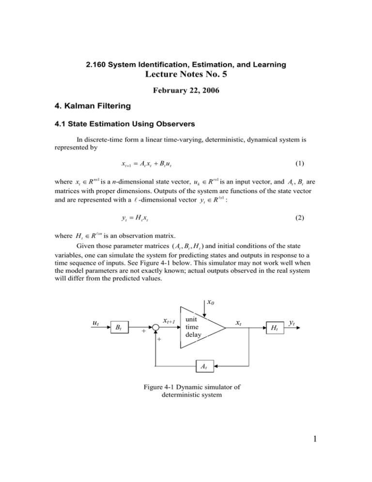
2.160 System Identification, Estimation, and Learning
Lecture Notes No. 5
February 22, 2006
4. Kalman Filtering
4.1 State Estimation Using Observers
In discrete-time form a linear time-varying, deterministic, dynamical system is
represented by
xt +1 = At xt + Bt u t
(1)
where xt ∈ R nx1 is a n-dimensional state vector, uk ∈ R rx1 is an input vector, and At , Bt are
matrices with proper dimensions. Outputs of the system are functions of the state vector
and are represented with a � -dimensional vector yt ∈ R �x1 :
yt = H t xt
(2)
.
where H t ∈ R �xn is an observation matrix
G
iven those parameter matrices ( At , Bt , H t ) and initial conditions of the state
variables, one can simulate the system for predicting states and outputs in response to a
ee F
-1 below. T
time seq
uence of inputs. S
igure 4
his simulator may not workwell when
the model parameters are not ex
actly k
nown;actual outputs observed in the real system
will differ from the predicted values.
x0
ut
Bt
xt+1
+
+
unit
time
delay
xt
Ht
yt
At
F
igure 4
-1 Dynamic simulator of
deterministic system
1
A dynamic state observer is a real-time simulator with a feedbackmechanism for
recursively correcting its estimated state based on the actual outputs measured from the
ee F
-2 below. Note that, unlik
real physical system. S
igure 4
e a standard feedbackcontrol
system, the discrepancy between the predicted outputs yı t and the actual outputs yt from
the real system are fed backto the model rather than the real physical system. Using a
feedbackgain matrixLt ∈ R nx� , the state observer is given by
xıt +1 = At xıt + Bt ut + Lt ( yt − yı t )
yı t = H t xıt
(3)
T
o differentiate the estimated state from the actual state of the physical system, the
estimated state residing in the real-time simulator is denoted xıt . With this feedbackthe
state of the simulator will follow the actual state of the real system, and thereby estimate
the state accurately. If the system is observable, convergence of the estimated state to the
actual state can be guaranteed with a proper feedbackgain. In other words, a stable
observer can forget its initial conditions;regardless of an initial estimated state xı0 , the
observer can produce the correct state as it converges. T
his is Luenberger’s S
tate
Observer for deterministic systems.
Real Physical System xt
yt
+
_
G
ain Lt
ut
xıt +1
+
Bt
+
+
xıt
unit
time
delay
xı0
At
Ht
yı t
Model
F
igure 4
-2 Luenberger’s state observer for
deterministic linear system
A special case of the above state observer is estimation of constant parameters θı .
ee eq
S
uation (17) in Chapter 2. Replacing the state transition matrixAt by the nx
n
identity matrixand setting inputs to zero leads to a recursive parameter estimation
formula in (2-17):
2
θı(t) = θı(t − 1) + Κ t ( y (t ) − yı(t ) )
(2-17)
T
he difference from the previous parameter estimation problem is that in state estimation
the state mak
es “state transition” as designated by the state transition matrixAt and the
uence. Both recursive parameter estimation
input matrixBt driven by an input time seq
and state estimation, however, are analogous;both based on the Prediction-ErrorCorrection formula.
Luenberger’s state observer is strictly for deterministic systems. In actual systems,
sensor signals are to some ex
tent corrupted with noise, and the state transition of the
actual process is to some ex
tent disturbed by noise. If stochastic properties of these noise
sources are available, state estimation may be performed more effectively than simply
using sensor signals as noise-free signals and estimating the sate based on noise-free state
transition model. Rudolph Kalman investigated this problem and developed the
celebrated Kalman F
urprisingly enough, Kalman did it 10 years before Luenberger
ilter. S
published his state observer paper.
T
o formulate this stochastic state estimation problem we need to use properties of
multivariable random processes, which will be summarized in the following section.
4.2 Multivariate Random Processes
Let us revisit S
ection 3.2 and consider the ensemble of time profiles again. Each of these
waveforms is a realization of random process X(t). (S
uch a random waveform can be
seen in your oscilloscope, when you increase the gain of a ground signal. T
he ensemble
of waveforms may be considered as a large collection of the same oscilloscope. If you
have hundreds of the same type of oscilloscopes, you have a collection of diverse ground
noise waveforms. T
hey come from the same ground signal, but the waveforms are all
different.) Now that stochastic properties of a single random process have been described
with the first and second order densities and auto-correlation functions, let us consider
multiple random processes, say X(t), Y(t), and Z(t), and characterize their properties. (In
the oscilloscope analogy, you can thinkabout two channels of signals, say channel 1 and
channel 2, shown on a single oscilloscope display. If there are a large number of the same
type of oscilloscopes displaying both channels, an ensemble of the two random processes
can be generated.)
A Multivariable random process : A vectorial random proces
S
tate variables = n-dimential vector
Observable outputs with multiple sensors
irst-order density fXYZ(x
F
t,yt,zt)
Covariance: Ensemble mean
⎡⎛ X (
t ) − m x (t) ⎞
⎤
⎟
⎥
⎢⎜
)
C XYZ (t ) =
E ⎢⎜ Y (t ) − m
Y (t ) ⎟( X (t ) − m x (t ) Y (t ) −
mY (t ) Z (t ) − mZ (t ) )⎥ (4
⎢⎣⎜⎝ Z (t ) − mZ (t) ⎟⎠
⎥⎦
If mx=my=mz=0
3
[
]
⎡ E X 2 (t )
E [X (t )Y (t )] E [X (t ) Z (t )]⎤
⎢
⎥
C XYZ (t ) = ⎢ E [X (t )Y (t )]
E Y 2 (t )
E [Y (t ) Z (t )]⎥
⎢ E [X (t ) Z (t )] E [Y (t ) Z (t )]
E Z 2
(t ) ⎥⎦
⎣
[
]
[
(5)
]
S
i
S
3
S
2
t
S
1
t
t
X (t ;S1 )
S
ix
x
t
t
t
S
1x
t
Ensemble
of waveforms
Y (t;S1 )
t
t
t1
t2
t1
t
Z (t ;S1 )
t2
t1
t
t2
t1
t
t2
F
igure 4
-3 Multivariable random processes
S
econd-order density:
ak
T
ing two time slices, t1 and t2, as shown in the above figure, the joint
probability density is given by: f X 1Y1Z1 X 2Y2 Z 2 ( xt1 , yt1 , z t1 , xt2 , yt2
, z t2
)
If mx=my=mz=0, the covariance is given by
⎡ E [X (t1 ) X (t 2 )] E [X (t1 )Y (t 2 )] E [X (t1
) Z (
t 2 )]⎤
C XYZ (t1 , t 2 ) = ⎢ E [Y (t1 ) X (t 2 )] E [Y (t1 )Y (t 2 )] E [Y (t1
) Z (t 2 )]⎥
⎥
⎢
⎢⎣ E [Z (t1 ) X (t 2 )] E [Z (t1 )Y (t 2 )] E [Z (t1
) Z (t 2 )]⎥⎦
(6)
Note that the first order covariance in eq
uation (5) can be viewed as a special case of the
second order covariance in eq
uation (6); t1
= t2
= t
.
4
4.3 State-Space Modeling of Random Processes
We ex
tend the state eq
uation given by (1) in the previous section to the one as a
multivariable random process. Namely, the state xt
∈ R nx1 is driven not only by the input
ut ∈ R rx1 but also by noise, which is a random process. Let wt ∈ R nx1
be a multivariable
random process, called “Process Noise”, driving the state through another matrix
Gt ∈ R nxn . T
he state eq
uation is then given by
xt+1 = At xt + Bt ut + Gt wt
(7)
S
ee F
igure 4
-4
.S
ince the process noise is a random process, the state xt driven by wt is a
he second term on the right hand side, Bt ut , is a deterministic term. In
random process. T
the following stochastic state estimation, this deterministic part of inputs is not important,
since its influence upon the state xt is completely predictable and hence it can be
herefore we often use the following state eq
eliminated without loss of generality. T
uation:
xt+1 = At xt + Gt wt
(8)
T
he outputs of the system are noisy, as long as they are measured with sensors.
Let vt ∈ R �x1 be another multivariable random process, called “Measurement Noise”,
super-imposed on a deterministic part of the output, the part completely determined by
the sate variable xt .
y
t = H t xt + vt
(9)
S
ee F
igure 4
-4
.S
ince measurement noise vt is a multivariable random process, the
outputs measured with sensor, too, are a multivariable random process.
wt
Gt
ut
+
Bt
vt
xt+1
+
+
unit
time
delay
xt
+
Ht
+
yt
At
F
igure 4
-4S
tate space representation of linear time varying system
with process noise and measurement noise
5
T
he stochastic properties of the process noise and measurement noise described
above are now characterized as multivariable random processes. It is a common practice
that the mean of noise is set to zero since, if the means are non-zero, the origins of the
state variables and the outputs can be shifted so that the mean of the noise is zero.
E[vt ] = 0
(10)
E[wt ] = 0
F
rom eq
uation (6), the covariance of measurement noise vt ∈ R �x1 is given by
T
CV (t , s ) = E[vt ⋅ vs ] ∈ R �x�
(11)
If the noise signals at any two time slices are uncorrelated,
T
CV (t , s ) = E[vt ⋅ vs ] =
0,
∀t ≠ s
(12)
the noise is called “White”. (We will discuss why this is called white later in the
following chapter.) Note that, if t=s, the above covariance is that of the first order density,
i.e. an auto-covariance.
T
CV (t ) = E[vt ⋅ vt ]
(13)
T
he diagonal elements of this matrixare variances of the individual output signals. If
those outputs are coupled through the state variables and the measurement matrixHt, (see
uation (9)), it is lik
eq
ely that the off-diagonal elements of the covariance matrixCv are
non-zero.
T
he process noise can be characterized in the same way. T
he covariance matrixis
then given by:
T
CW (
t , s ) = E[ wt ⋅ ws ] ∈ R nxn
(14
)
F
urthermore, the correlation between the process noise and the measurement noise may
ex
his can be
ist, if both are generated in part by the same disturbance source. T
represented with the covariance matrixgiven by:
T
CWV (t , s ) = E[ wt ⋅ vs ] ∈ R nx�
(15)
Usually the covariance between the process and measurement noises is zero.
4.4 Framework of the Kalman Filter
Consider a dynamical system given by eq
uations (8) and (9),
6
xt+1 = At xt + Gt wt
(8)
yt = H t xt + vt
(9)
where xt ∈ R nx1 , yt ∈ R �x1 , wt ∈ R nx1 , vt ∈ R �x1 , At , Gt ∈ R n×n , and H t ∈ R �xn . Assume
that the process noise wt and the measurement noise vt have zero mean values,
E[wt]=0, E[vt]=0.
(16)
and that they have the following covariance matrices:
⎧0
T
CV (t , s ) = E[vt ⋅ vs ] = ⎨
⎩ Rt
⎧0
T
CW (t , s ) = E[ wt ⋅ ws ] = ⎨
⎩Qt
T
CWV (t , s ) = E[ wt ⋅ vs ] = 0
∀t ≠ s
(17)
∀t = s
∀t ≠ s
(18)
∀t = s
∀t , ∀s
(19)
where matrixRt is of �x
� , and is positive definite, and matrixQt ∈ R nxn is positive semidefinite.
Uncorrelated
w
Process
Noise
t
s
time
Uncorrelated
v
Measurement
(S
ensor) Noise
time
F
igure 4
-5 Noise characteristics
Optimal State Estimation Problem
Obtain an optimal estimate of state vector xt based on measurements yt, t = 1,2,…t,
that minimizes the mean sq
uared error:
[
]
T
J t = E ( xı t − xt ) ( xı t − xt )
(20)
7
subject to the state eq
uation (8) and the output eq
uation (9) with white, uncorrelated
process and measurement noises of zero mean and the covariant matrices given by
uations (16) - (18). (Necessary initial conditions are assumed.)
eq
Rudolf E. Kalman solved this problem around 1960.
Kalman F
ilter: two major points of his seminal workin 1960.
I)
If we assume that the optimal filter is linear, then the Kalman filter is the state
estimator having the smallest unconditioned error covariance among all linear
filters.
If we assume that the noise is G
aussian, then the Kalman filter is the optimal
minimum variance estimator among all linear and non-linear filters.
II)
4.5 The Discrete Kalman Filter as a Linear Optimal Filter
F
igure 4
-6 depicts the outline of the discrete Kalman filter,
y1
yt-2
yt-1
All k
nowledge
up to t-1
yt
time
Estimation
error
Estimate
output
yı t = H t xıt |t −1
S
tate Estimate
xıt−1
a priori
estimate
xıt | t −1
Ex
pected state transition
based on the model
Correction
to state
estimate
a posteriori
estimate
xıt
F
igure 4
-6 Outline of the Kalman filter algorithm
Expected state transition
F
rom (8), we k
now how the previous estimate xıt −1 will mak
e a transition
xt ⇐ At −1 xt −1 +
Gt −1wt −1 ;Let’s write this as
xı
t t −1
T
ransition from estimated state at time t-1, xıt −1
8
xıt t −1 = E[ At −1 xıt −1 + Gt −1wt −1 ]
= At −1 xıt −1 + Gt −1E[
wt −1 ]
Ex
pected state based on xıt −1
Estimated output
F
orm (9) and (10)
yıt = H t xıt t −1 Note E[vt]=0
(21)
(22)
Correction of the state estimate
Assimilating the new measurement yt, we can update the state estimate in
proportion to the output estimation error.
xıt = xıt t −1 + K t ( yt − H t xıt t −1 )
(23)
Eq
uation (23) provides a structure of linear filter in recursive form. K t ∈ R n×l is a gain
matrixto be optimized so that the mean sq
pected value of error) of state
uared error (ex
estimation may be minimized.
A more general form of linear filter is
xıt = K t1 xıt t −1 + K t 2 yt
(24
)
Both (23) and this form provide the same result.
9