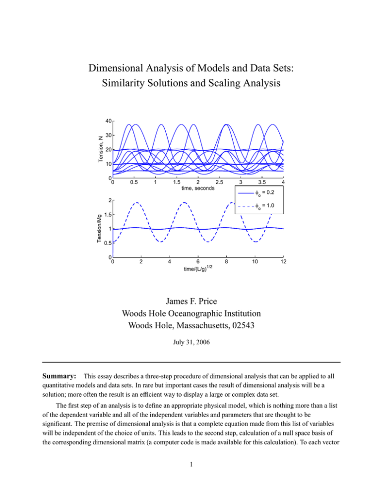
Dimensional Analysis of Models and Data Sets:
Similarity Solutions and Scaling Analysis
Tension, N
40
30
20
10
0
0
0.5
1
1.5
2
2.5
time, seconds
3
3.5
4
φ = 0.2
o
2
φ = 1.0
Tension/Mg
o
1.5
1
0.5
0
0
2
4
6
time/(L/g)1/2
8
10
12
James F. Price
Woods Hole Oceanographic Institution
Woods Hole, Massachusetts, 02543
July 31, 2006
Summary: This essay describes a three-step procedure of dimensional analysis that can be applied to all
quantitative models and data sets. In rare but important cases the result of dimensional analysis will be a
solution; more often the result is an efficient way to display a large or complex data set.
The first step of an analysis is to define an appropriate physical model, which is nothing more than a list
of the dependent variable and all of the independent variables and parameters that are thought to be
significant. The premise of dimensional analysis is that a complete equation made from this list of variables
will be independent of the choice of units. This leads to the second step, calculation of a null space basis of
the corresponding dimensional matrix (a computer code is made available for this calculation). To each vector
1
of the null space basis there corresponds a nondimensional variable, the number of which is less than the
number of dimensional variables. The nondimensional variables are themselves a basis set and in most cases
their form is not determined by dimensional analysis alone.
The third and in some respects most interesting step is to choose an optimal form for the basis set. One
very useful strategy is to nondimensionalize the dependent variable by a physically motivated ’zero order’
solution. When carried to completion, this leads naturally to a scaling analysis in which the nondimensional
variables of a model equation are O(1) in some relevant limit. Scaling analysis is often an essential first step
in an approximation method. The remaining nondimensional variables can then be formed in ways that define
the geometry of the problem or that correspond to the ratios of terms in a model equation, e.g., the Reynolds
number or Froude number often arise in models of geophysical fluid dynamics.
Cover page graphic: The tension in the line of a simple pendulum computed by a model for 16 different
combinations of length, mass, gravitational acceleration and initial displacement, the angle, o . The upper
graph shows the tension as a function of time in dimensional units, and the lower graph is the same data
shown in non-dimensional units. The 16 separate solutions collapse to just two, depending upon o and time
alone. This kind of data compression illustrates an important advantage to the use of nondimensional
variables and dimensional analysis that is described further in Section 4.3.
Contents
1 About dimensional analysis
4
1.1
The goal and the plan . . . . . . . . . . . . . . . . . . . . . . . . . . . . . . . . . . . . . . .
4 1.2
About this essay . . . . . . . . . . . . . . . . . . . . . . . . . . . . . . . . . . . . . . . . . .
5 2 Models of a simple pendulum
5
2.1
A physical model . . . . . . . . . . . . . . . . . . . . . . . . . . . . . . . . . . . . . . . . .
6 2.2
A mathematical model . . . . . . . . . . . . . . . . . . . . . . . . . . . . . . . . . . . . . .
6 2.3
Models generally . . . . . . . . . . . . . . . . . . . . . . . . . . . . . . . . . . . . . . . . .
8 3 An informal dimensional analysis
9
3.1
Invariance to a change of units . . . . . . . . . . . . . . . . . . . . . . . . . . . . . . . . . .
9 3.2
Natural units . . . . . . . . . . . . . . . . . . . . . . . . . . . . . . . . . . . . . . . . . . . .
11 3.3
Extra and omitted variables . . . . . . . . . . . . . . . . . . . . . . . . . . . . . . . . . . . .
12 4 A basis set of nondimensional variables
13
4.1
The mathematical problem . . . . . . . . . . . . . . . . . . . . . . . . . . . . . . . . . . . .
13 4.2
The null space . . . . . . . . . . . . . . . . . . . . . . . . . . . . . . . . . . . . . . . . . . .
15 4.3
A basis set for the simple, inviscid pendulum . . . . . . . . . . . . . . . . . . . . . . . . . .
16
2
5 The viscous pendulum
18
5.1
A physical model of the viscous pendulum . . . . . . . . . . . . . . . . . . . . . . . . . . . .
19
5.2
Drag on a moving sphere . . . . . . . . . . . . . . . . . . . . . . . . . . . . . . . . . . . . .
20 5.2.1
Zero order solution . . . . . . . . . . . . . . . . . . . . . . . . . . . . . . . . . . . .
21 5.2.2
The other nondimensional variables: remarks on the Reynolds number . . . . . . . . .
22
5.3
A numerical simulation . . . . . . . . . . . . . . . . . . . . . . . . . . . . . . . . . . . . . .
23 5.4
An approximate model of the decay rate . . . . . . . . . . . . . . . . . . . . . . . . . . . . .
25
6 A similarity solution for diffusion in one dimension
27
6.1
Honing the physical model . . . . . . . . . . . . . . . . . . . . . . . . . . . . . . . . . . . .
28 6.2
A similarity solution . . . . . . . . . . . . . . . . . . . . . . . . . . . . . . . . . . . . . . .
28 7 Scaling analysis
31
7.1
A nonlinear projectile problem . . . . . . . . . . . . . . . . . . . . . . . . . . . . . . . . . .
31 7.2
Small parameter ! small term? . . . . . . . . . . . . . . . . . . . . . . . . . . . . . . . . .
34 7.3
Scaling the dependent variable . . . . . . . . . . . . . . . . . . . . . . . . . . . . . . . . . .
36 7.4
Approximate and iterated solutions . . . . . . . . . . . . . . . . . . . . . . . . . . . . . . . .
37
8 Summary and closing remarks
39
3
MIT OpenCourseWare
http://ocw.mit.edu
Resource: Online Publication.Fluid Dynamics
James Price
The following may not correspond to a particular course on MIT OpenCourseWare, but has been
provided by the author as an individual learning resource.
For information about citing these materials or our Terms of Use, visit: http://ocw.mit.edu/terms.