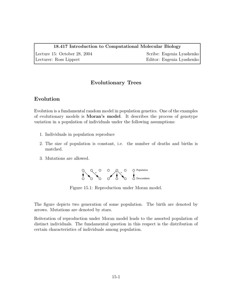
18.417 Introduction to Computational Molecular Biology
Lecture 15: October 28, 2004
Lecturer: Ross Lippert
Scribe: Eugenia Lyashenko
Editor: Eugenia Lyashenko
Evolutionary Trees
Evolution
Evolution is a fundamental random model in population genetics. One of the examples
of evolutionary models is Moran’s model. It describes the process of genotype
variation in a population of individuals under the following assumptions:
1. Individuals in population reproduce
2. The size of population is constant, i.e. the number of deaths and births is
matched.
3. Mutations are allowed.
Population
*
*
Descendants
Figure 15.1: Reproduction under Moran model.
The figure depicts two generation of some population. The birth are denoted by
arrows. Mutations are denoted by stars.
Reiteration of reproduction under Moran model leads to the assorted population of
distinct individuals. The fundamental question in this respect is the distribution of
certain characteristics of individuals among population.
15-1
15-2
Lecture 15: October 28, 2004
In the absence of mutations we can end up with the population homogeneous with
respect to some trait:
1
1
1
1
1
1
1
1
1
1
Figure 15.2: No mutations.
When some mutation occur, we can describe them by bit flipping. After certain
amount of time we get a random distribution of a trait.
1
1
1
1
*
1
1
*
0
1
0
1
Figure 15.3: Mutations allowed.
Figure 15.4: Moran model.
Coalescent
There are different probabilistic models that deal with above situation. One of them
is the coalescent analysis.
15-3
Lecture 15: October 28, 2004
We use simplified, modified Moran model. Based on the present data it analyzes
retrospectively the past events. Based on the present generation it deduces what past
events might be and what are relations with ancestors.
We start with the present time population and reverse the process of reproduction
in Moran model. We randomly pick ancestors to the current individuals, keeping the
size of population constant. We the repeat the process. This way we build a Moran
Figure 15.5: Going backwards.
model with some random topology.
Fix a subset of individuals and select a random topology. If we go farther and farther
back in time we get a tree.
Figure 15.6: A tree.
The coalescent has some limitations because in real world:
• Parents can be mixed.
• There can be more complicated modifications.
• Genetic recombination can occur.
Building trees
Definition 1 Taxonomy is the science of classification of organisms.
15-4
Lecture 15: October 28, 2004
There are two main approaches to taxonomy.
Phenetic Phenetics approach is based on the overall similarity between organisms.
The main criterion for clustering species is the current similarity according to
all possible traits.
Cladistics Considers the various possible phylogenetic trees and chooses from among
these the best possible tree.
The two approaches can give different phylogenetic trees:
The Phenetic & Cladistic criteria of relationship differ if evolutionary rates
are unequal
Lizard Crocodile
Bird
Birds have evolved quickly
since their divergence
from crocodiles
Lizard
Lizard
Crocodile
Crocodile
Bird
Bird
Cladistic
Phenetic
Adapted from Figure 15.7: Phenetic vs Cladistic.
Phylogenetic tree of life
Bacteria
Archaea
Eucarya
Green Filamentous
bacteria
Spirochetes
Proteobacteria
Cyanobacteria
Planctomyces
Bacteroides
Cytophaga
Gram
positives
Slime molds Animals
Methanosarcina
Fungi
Entamoebae
Methanobacterium
Plants
Halophiles
Methanococcus
Ciliates
T. celer
Flagellates
Thermoproteus
Trichomonads
Pyrodictium
Microsporidia
Thermotoga
Aquifex
Adapted from Figure 15.8: Phylogenetic Tree of Life.
Diplomonads
15-5
Lecture 15: October 28, 2004
Molecular Clock Hypothesis
Introduced by Pauling and Zuckerkandl, the Molecular Clock Hypothesis states that
mutations in certain regions of genome accumulate at a rate linearly proportional to
time.
The diagram below shows the difference in DNA between some species versus time
starting from millions years ago when organisms first were found in fossils. Compare
Nucleotide Substitutions
100
75
50
25
0
0
25
50
75
100
125
Millions of Years Ago
Adapted from Figure 15.9: Mutations allowed.
DNA of today’s organisms with ancient. This means that the amount of molecular
change between two species measures how long ago they shared a common ances­
tor. Molecular differences between species are therefore used to infer phylogenetic
relations.
There are several ways to observe molecular clock.
1. Mutations in mitochondrial DNA (mtDNA) are used as molecular clock in many
systematic studies.
2. Neutral mutation in the noncoding region of gene.
3. Mutations in ribosomal DNA (rDNA).
Trees in biology
Phylogenetic trees illustrate the evolutionary relationship between species. We con­
sider trees whose nodes have degree 3 each. Each node represents some species.
15-6
Lecture 15: October 28, 2004
African
Non-African
Common origin of European, Asian,
Australian, & New World peoples
38,500 +- 1,500 yr ago
82
100
100
*
98
98
98
1 Chukchi
2 Australian
3 Australian
4 Piman
5 Italian
6 PNG Highland
7 PNG coast
8 PNG Highland
9 Georgian
10 German
11 Uzbek
12 Saam
13 Crimean Tatar
14 Dutch
15 French
16 English
17 Samoan
18 Korean
19 Chinese
20 Asian Indian
21 Chinese
22 PNG coast
23 Australian
24 Evenki
25 Buriat
26 Khirgiz
27 Warao
28 Warao
29 Siberian Inuit
30 Guarani
31 Japanese
32 Japanese
33 Mkamba
34 Ewondo
35 Bamileke
36 Lisongo
37 Yoruba
38 Yoruba
39 Mandenka
40 Effik
41 Effik
50 Mbuti
42 Ibo
43 Ibo
44 Mbenzele
45 Biaka
46 Biaka
47 Mbenzele
48 Kikuyu
49 Hausa
53 San
51Mbuti
52 San
Adapted from Figure 15.10: Human mtDNA tree.
External nodes correspond to present time species. Internal nodes represent their an­
cestors. External nodes called leaves represent the present time species. Each node
represents an even of splitting one species from another.
Ancestor
Descendants
Figure 15.11: Tree node
Multiple splitting can also be thought of as single splitting in a short time interval.
Unrooted tree is a tree without a specified root. An unrooted phylogenetic tree is a
reflection of our ignorance as to where the common ancestor lies.
Given a tree we can form a distance matrix whose entries are distances between pairs
of leaves. Distance function on the tree should satisfy the triangle inequality
d(A, B) + d(B, C) � d(A, C).
Lecture 15: October 28, 2004
15-7
Distance based tree reconstruction
The problem of reconstructing a tree from its distance matrix naturally arises. Given
all pairwise distances in the tree we need to reconstruct the tree.
Input Distance matrix from some unknown tree.
Output Tree compatible with a given distance matrix.
This problem is solved using additive tree reconstruction. One way to do this
is to find a pair of neighboring leaves, that is leaves that have the common parent
vertex.
If i and j are neighboring leaves and k is their parent, then for any other leave m we
have:
d(i, m) + d(j, m) − d(i, j)
d(k, m) =
.
2
Having found neighboring pair i, j we replace them by their parent k. Then we update
the distance matrix using the above formula. Hence if we had sequence of neighbors
relations, we could reconstruct the tree. Determining which leaves are neighbors is
however a nontrivial task.
Another approach to tree reconstruction is shortening of edges. We choose a small
number x, for example x = 1. If we decrease the length of each edge leaving to leaves1
by x, then all distances will decrease by 2x.
Updating the distance matrix according to rule d � d − 2x, we obtain a new matrix
corresponding to a tree with shorter hanging edges.
If there is a triple of leaves i, j, k such that d(i, j) + d(j, k) = d(i, k) in the updated
distance matrix, then leaves i, j, k lie on the single path. Hence j is attached by an
edge of length 0 to the path from i to k. We can then throw out vertex j and continue.
The algorithm which is based on above analysis is presented in [1][p. 364].
To discern additive distance matrix from non-additive ones we use
Test for additiveness [Bunneman].
Given any four points we can rename them A, B, C, D so that:
d(A, B) + d(C, D) = d(A, C) + d(B, D) � d(A, D) + d(B, C).
1
such edges are called hanging
15-8
Lecture 15: October 28, 2004
Figure 15.12: Tree node
15.0.1
Approximate additive tree reconstruction
But it is a fact, that the evolutionary clock is running differently for different species
and even for different regions in a protein sequence. Hence some distances matrices
we obtain are not additive.
Since not all distance matrices turn out to be additive, we are facing the following
problem:
Given a distance matrix, find the nearest additive tree?
This problem is NP-complete. However, there are also several algorithms that deal
with above problem.
UPGMA Algorithm (Unweighted Pair Group Method with Arithmetic mean).
UPMGA is a variant of Hierarchical Clustering. It assigns heights to vertices of
constructed trees. The leave with the most mutations (the oldest) has the highest
height. The height serves as a molecular clock in this case.
Neighbor Joining
Intuition behind this algorithm was mentioned above: if we identify two neighbors in
a tree, join them together. Then repeat until done.
We’re interested in pairs, for which not only the distance between them is smallest,
but also the distance to the rest points is largest.
The algorithm is following:
1. For each i define
ui =
�
d(i, k)
.
n−2
k=i
�
15-9
Lecture 15: October 28, 2004
2. Now take the pair i, j for which d(i, j) − ui − uj is minimal. Designate i, j to
be neighbors and join them in a cluster n.
3. Recompute the distance matrix:
d(n, k) =
d(i, k) + d(j, k) − d(i, j)
.
2
4. Repeat until finished.
Character-based methods
Character-based methods take as input an n × m matrix where n is the number of
species and m is the number of characters. The goal is a tree whose leaves correspond
to n rows. The parsimony problem, which arises in this respect, is to minimize the
number of evolutionary events to put on the tree.
Large Parsimony Problem2
Input An n × m matrix M describing n species, each representing by an m-character
string.
Output A tree T with n leaves labeled by n rows of M , and a labeling of the internal
vertices of T such that the parsimony score is minimized over all possible trees
and all labelings.
References
[1] N.C. Jones, P.A. Pevzner, Introduction to Bionformatics Algorithms, A Bradford
Book, The MIT Press, Cambridge, 2004.
2
[1][p. 374]