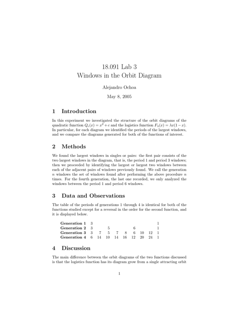
18.091 Lab 3
Windows in the Orbit Diagram
Alejandro Ochoa
May 8, 2005
1
Introduction
In this experiment we investigated the structure of the orbit diagrams of the
quadratic function Qc (x) = x2 + c and the logistics function Fλ (x) = λx(1 − x).
In particular, for each diagram we identified the periods of the largest windows,
and we compare the diagrams generated for both of the functions of interest.
2
Methods
We found the largest windows in singles or pairs: the first pair consists of the
two largest windows in the diagram, that is, the period 1 and period 3 windows;
then we proceeded by identifying the largest or largest two windows between
each of the adjacent pairs of windows previously found. We call the generation
n windows the set of windows found after performing the above procedure n
times. For the fourth generation, the last one recorded, we only analyzed the
windows between the period 1 and period 6 windows.
3
Data and Observations
The table of the periods of generations 1 through 4 is identical for both of the
functions studied except for a reversal in the order for the second function, and
it is displayed below.
Generation
Generation
Generation
Generation
4
1
2
3
4
3
3
3
6
7
14
5
5
10
7
14
8
16
6
6
12
10
20
12
24
1
1
1
1
Discussion
The main difference between the orbit diagrams of the two functions discussed
is that the logistics function has its diagram grow from a single attracting orbit
1
into chaos from left to right, while the quadratic function does it from right to
left. As our data shows, the structure of the largest windows is the same for
both functions, and visually the two diagrams are strikingly similar if we reflect
either on the x­axis.
A pattern stands out in the table of our data: for each generation, the values
of the periods in the sequence are half of the values of the rightmost periods
of the following generation’s sequence, without including 1. For example, note
that except for 1, each of the entries on the row of generation 4 is the double
of the value of the entry above it, on the generation 3 row, and that 3, 5, and
6 are the halves of 6, 10, and 12 respectively.
Assuming the pattern just discussed holds in general, then we expect the
rightmost values of the table for generation 5 to be
Generation 5
12
28
20
28
32
24
40
48
1.
However, it is not clear how the rest of the numbers in the table could be
generated.
2