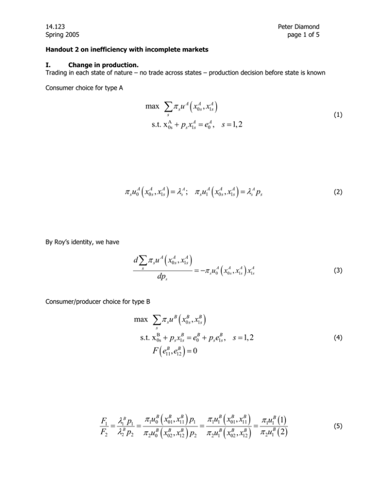
14.123
Spring 2005
Peter Diamond
page 1 of 5
Handout 2 on inefficiency with incomplete markets
I.
Change in production.
Trading in each state of nature – no trade across states – production decision before state is known
Consumer choice for type A
max
∑s π su A ( x0As , x1As )
(1)
s.t. x + p x = e , s = 1, 2
A
0s
A
s 1s
A
0
π su0A ( x0As , x1As ) = λsA ; π s u1A ( x0As , x1As ) = λsA ps
(2)
By Roy’s identity, we have
d ∑ π s u A ( x0As , x1As )
s
dps
= −π s u0A ( x0As , x1As ) x1As
(3)
Consumer/producer choice for type B
max
∑s π su B ( x0Bs , x1Bs )
B
+ ps x1Bs = e0B + ps e1Bs , s = 1, 2
s.t. x 0s
(4)
F ( e11B , e12B ) = 0
B
B
B
B
B
B
B
F1 λ1B p1 π1u0 ( x01 , x11 ) p1 π 1u1 ( x01 , x11 ) π1u1 (1)
=
=
=
=
B
B
B
F2 λ2B p2 π 2u0B ( x02
, x12B ) p2 π 2u1B ( x02
, x12B ) π 2u1 ( 2 )
(5)
14.123
Spring 2005
Peter Diamond
page 2 of 5
Market clearance
x1A ( ps , e0A ) + x1B ( ps , e0B + ps e1Bs ) = e1Bs
(6)
ps = p ( e1Bs )
(7)
de12
F
=− 1
de11
F2
(8)
x1As = − ( x1Bs − e1Bs )
(9)
implying:
Impact of deviation from production decision
de12
d
A
A
A
A
A
′ B
′ B
B ∑ π s u ( s ) = −π 1u0 (1) x11 p ( e11 ) − π 2u0 ( 2 ) x12 p ( e12 )
de11 s
de11
⎡
π u A ( 2) A
de12 ⎤
= −π u (1) ⎢ x11A p′ e11B + 2 0A
x12 p′ e12B
⎥
π1u0 (1)
de11 ⎥⎦
⎢⎣
( )
A
1 0
( )
⎡ B
⎤
π 2u0B ( 2 ) B B
d
B
B
B
B
B de12
′
′
π
π
=
−
−
+
−
u
s
u
1
x
e
p
e
x
e
p
e
(
)
(
)
⎢
⎥
(
)
(
)
(
)
(
)
s
1 0
11
11
11
12
π1u0B (1) 12 12
de11 ⎦⎥
de11B ∑
s
⎣⎢
⎡ A
⎤
π 2u0B ( 2 ) A
B
B
B de12
′
′
= π 1u0 (1) ⎢ x11 p e11 +
x
p
e
⎥
12
12
π 1u0B (1)
de11 ⎥⎦
⎣⎢
( )
( )
(10)
(11)
14.123
Spring 2005
Peter Diamond
page 3 of 5
II. Change in production with redistribution
We now add redistribution in numeraire good, at the same level in both states of nature.
This changes market clearance to:
implying:
x1A ( ps , e0A − T ) + x1B ( ps , e0B + T ) = e1Bs
(12)
ps = p ( e1Bs , T )
(13)
∂x1A ∂x1B
−
∂ps
∂I
∂I
= A
A
B
∂x
∂x
∂x B
∂T ∂x1
− T1 1 + 1 + ( e1Bs + T1 ) 1
∂p
∂I
∂p
∂I
(14)
⎧ ∂x1A ∂x1B ⎫
ps ⎨
−
⎬
∂I
∂I ⎭
∂ps
⎩
=
∂x A ∂x B
∂x B
∂T1 ∂x1A
− T1 1 + 1 + ( e1Bs + T1 ) 1
∂p
∂I
∂p
∂I
(15)
Note that
As long as the income derivatives of A and B are different, these are nonzero. Also the demand
derivatives are evaluated at different prices and incomes in the different states.
14.123
Spring 2005
Peter Diamond
page 4 of 5
Starting with zero transfers, consider a derivative change in the two transfers, satisfying (for some
constant k).
dT1 = kdT0
(16)
This implies that
⎧ ∂x1A ∂x1B ⎫
(1 + kps ) ⎨ − ⎬
∂I ⎭
∂ps
dps ∂ps
⎩ ∂I
≡
+k
= A
A
B
∂x
∂x
∂x B
dT0 ∂T0
∂T1 ∂x1
− T1 1 + 1 + ( e1Bs + T1 ) 1
∂p
∂I
∂p
∂I
(17)
≡ (1 + kps ) α s
We want to evaluate the impact of a redistribution on expected utilities in equilibrium.
d
π s u A ( s ) = −∑ π s ( u0A ( s ) + ku1A ( s ) )
∑
dT0 s
s
−π 1u0A (1) x11A
dp1
dp
− π 2u0A ( 2 ) x12A 2
dT0
dT0
(18)
⎡
⎤
π 2u0A ( 2 )
A
A
+
kp
= −π u (1) ⎢(1 + kp1 ) (1 + x11α1 ) +
+
1
1
α
x
(
)
⎥
(
)
12
2
2
π 1u0A (1)
⎣⎢
⎦⎥
A
1 0
Similarly, using the same substitutions as in (11),
⎡
⎤
π 2u0B ( 2 )
d
A
B
B
π
π
+
=
+
1
x
α
+
u
s
u
1
1
kp
1 + kp2 ) (1 + x12Aα 2 )⎥
(
)
(
∑
11 1 )
s
1 0 ( ) ⎢(
1)(
B
π1u0 (1)
dT0 s
⎢⎣
⎥⎦
(19)
14.123
Spring 2005
Peter Diamond
page 5 of 5
Generically we have different prices and demands in the two states and different marginal rates of
substitution for the two agents. The aim is to find a constant, k, so that the changes in transfers leave
both of them better off or both worse off (in which case we reverse the direction of transfers). This may
be possible – this model does not fit the Inefficiency Theorem. Contrasting (18) and (19) to (10) and
(11), we have an extra degree of freedom in seeking a Pareto gain.
For a Pareto gain, we need to find a value of k such that (18) and (19) are both positive or both
negative (calling for a reversal of the direction of redistribution). This requires
(1 + kp2 ) (1 + x12Aα 2 ) π 2u0B ( 2 )
π 2u0A ( 2 )
<−
<
π 1u0A (1)
(1 + kp1 ) (1 + x11Aα1 ) π1u0B (1)
(20)
(1 + kp2 ) (1 + x12Aα 2 ) π 2u0B ( 2 )
π 2u0A ( 2 )
>−
>
π 1u0A (1)
(1 + kp1 ) (1 + x11Aα1 ) π 1u0B (1)
(21)
or