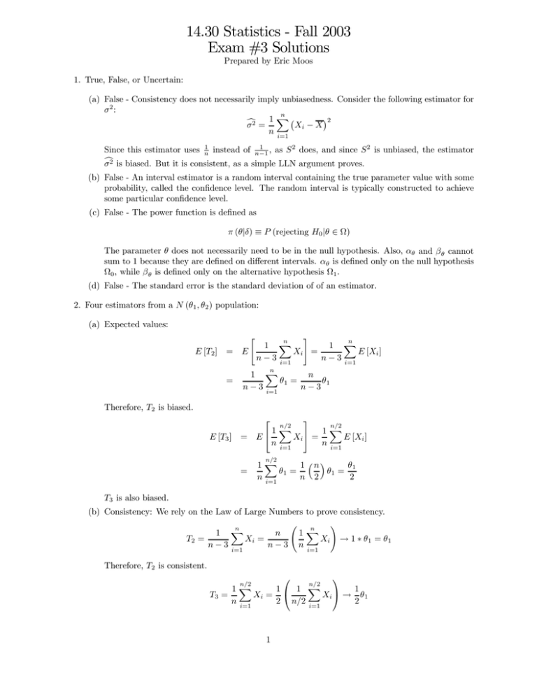
14.30 Statistics - Fall 2003
Exam #3 Solutions
Prepared by Eric Moos
1. True, False, or Uncertain:
(a) False - Consistency does not necessarily imply unbiasedness. Consider the following estimator for
σ2 :
n
X
¢2
¡
c2 = 1
σ
Xi − X
n i=1
1
Since this estimator uses n1 instead of n−1
, as S 2 does, and since S 2 is unbiased, the estimator
c2 is biased. But it is consistent, as a simple LLN argument proves.
σ
(b) False - An interval estimator is a random interval containing the true parameter value with some
probability, called the confidence level. The random interval is typically constructed to achieve
some particular confidence level.
(c) False - The power function is defined as
π (θ|δ) ≡ P (rejecting H0 |θ ∈ Ω)
The parameter θ does not necessarily need to be in the null hypothesis. Also, αθ and β θ cannot
sum to 1 because they are defined on different intervals. αθ is defined only on the null hypothesis
Ω0 , while β θ is defined only on the alternative hypothesis Ω1 .
(d) False - The standard error is the standard deviation of of an estimator.
2. Four estimators from a N (θ1 , θ2 ) population:
(a) Expected values:
"
#
n
n
1 X
1 X
E [T2 ] = E
Xi =
E [Xi ]
n − 3 i=1
n − 3 i=1
n
=
n
1 X
θ1 =
θ1
n − 3 i=1
n−3
Therefore, T2 is biased.
⎡
⎤
n/2
n/2
X
1
1X
⎣
⎦
E [T3 ] = E
Xi =
E [Xi ]
n i=1
n i=1
1X
1 ³n´
θ1
θ1 =
θ1 =
n i=1
n 2
2
n/2
=
T3 is also biased.
(b) Consistency: We rely on the Law of Large Numbers to prove consistency.
!
à n
n
1 X
n
1X
T2 =
Xi =
Xi → 1 ∗ θ1 = θ1
n − 3 i=1
n − 3 n i=1
Therefore, T2 is consistent.
⎞
⎛
n/2
n/2
1X
1⎝ 1 X ⎠
1
T3 =
Xi =
Xi → θ1
n i=1
2 n/2 i=1
2
1
Therefore, T3 is inconsistent.
n
1 X
1
Xi =
T4 = 2
n i=1
n
Ã
n
1X
Xi
n i=1
!
→ 0 ∗ θ1 = 0
Therefore, T4 is inconsistent.
(c) Variancs of estimators:
£ ¤ θ2
V ar [T1 ] = V ar X =
n
and
⎤
n/2
n/2
X
1 X
1
⎦
⎣
Xi = 2
V ar [Xi ]
V ar [T3 ] = V ar
n i=1
n i=1
⎡
=
n/2
1 X
1 ³n ´
θ2
θ2 = 2
θ2 =
2
n i=1
n 2
2n
Therefore, V ar [T3 ] < V ar [T1 ].
(d) Actual data:
x =
s2
=
=
£ ¤
V ar X =
1
9
(1 + 5 + 3) = = 3
3
3
i
1 h
2
(1 − 3) + (5 − 3)2 + (3 − 3)2
3−1
1
(8) = 4
2
θ2
3
For method of moments estimation,
x = E [X] = θ1
θb1 = x
n
£ ¤
1X 2
x = E X 2 = θ2 + θ21
n i=1
n
θb2
=
1 X 2 b2
x − θ1
n i=1
n
=
1X 2
x − x2
n i=1
= 8/3
3. Maximum likelihood estimation:
(a) In order to calculate the MLE of the mean, we need to calculate the mean of the distribution.
E [Y ] =
Z1
0
=
yθy
θ−1
dy =
Z1
θy θ dy
0
¯1
¯
θ
θ
θ+1 ¯
y ¯ =
θ+1
θ+1
0
θ
is simplfied by the invariance property of MLE’s; we need only
Calculating the MLE of θ+1
b
b
calculate the MLE of θ, θ, and then use b θ as the MLE. To calculate the MLE, we need the joint
θ+1
2
pdf of the sample, now known as the likelihood function; it will be convenient to use the natural
logarithm of the likelihood function.
ln f (y|θ) = ln
n
Y
i=1
n
X
=
i=1
n
X
f (yi |θ) =
ln f (yi |θ)
i=1
n
X
¡
¢
ln θyiθ−1 =
= n ln θ + (θ − 1)
i=1
n
X
[ln θ + (θ − 1) ln yi ]
ln yi
i=1
The first-order condition of the maximization problem is the following:
n
n X
ln yi
+
θ i=1
= 0
b
θ =
−n
n
X
ln yi
i=1
Therefore,
−n
b
θ
µ
b =
b
θ+1
=
n
X
i=1
=
−n
n
X
ln yi
i=1
−n
1+ X
n
ln yi
i=1
ln yi − n
(b) Considering the limited information constraint, the probability that we observe 0.4 is the following:
P (Y ≤ 0.4) =
0.4
Z
θy θ−1 dy
0
=
¯0.4
y θ ¯0 = (0.4)θ
Letting m be the number of observations that are not equal to 0.4 (hence, n − m observations are
0.4), the new likelihood function is the following:
f (y|θ) =
n
Y
i=1
(n−m)θ
ln f (yi |θ) = (0.4)
à m !θ−1
Y
(n−m)θ n
= (0.4)
θ
yi
m
Y
θyiθ−1
i=1
i=1
with the following log-likelihood function:
ln f (y|θ) = (n − m) θ ln (0.4) + m ln θ + (θ − 1)
3
m
X
i=1
ln yi
where The first-order condition for this new, limited information MLE problem is the following:
m
m X
+
(n − m) ln (0.4) +
ln yi
θ
i=1
= 0
b
θ =
−m
(n − m) ln (0.4) +
m
X
ln yi
i=1
4. Given the distributions of the X sample and Y sample, we can conclude that
µ
¶
σ2X
X ∼ N µX ,
nX
and
Y ∼N
µ
σ2
µY , Y
nY
¶
Therefore,
X +Y
X + Y − µX + µY
q 2
σX
σ 2Y
nX + nY
µ
¶
σ2
σ2
∼ N µX + µY , X + Y
nX
nY
∼ N (0, 1)
since the samples are independent. In order to construct the confidence interval, we do the following:
⎛
⎞
X
+
Y
−
µ
−
µ
q 2 X 2 Y ≤ 1.96⎠
95% = P ⎝−1.96 ≤
σX
σY
nX + nY
⎞
⎛
s
s
2
2
2
2
σ
σ
σ
σ
X
X
+ Y ≤ X + Y − µX − µY ≤ 1.96
+ Y⎠
= P ⎝−1.96
nX
nY
nX
nY
⎛
⎞
s
s
2
2
2
2
σ
σ
σ
σ
X
X
P ⎝X + Y − 1.96
+ Y ≤ µX + µY ≤ X + Y + 1.96
+ Y⎠
nX
nY
nX
nY
5. Hypothesis testing:
(a) Let us consider a simple two-sided test of the following hypotheses:
H0
H1
: µ=0
: µ=
6 0
For a simple two-sided test, we reject H0 if
|x| > k
(Typically, our decision rule will be something of the form "reject H0 if x > k1 or if x < k2 ."
But since the normal and t−distributions, which we will be using, are symmetric, we know that
k1 = k2 = k. Since the distribution is unknown, we must hope that some limiting result helps us.
Fortunately, the Central Limit Theorem assures us that X is asymptotically normal. A sample
size of 100 should be (hopefully) sufficiently large to assure normality.
X −µ
√ ∼ N (0, 1)
σ/ n
4
Although we do not know σ 2 , this is no problem. We can estimate it using s2 . Although this
might suggest to you that we must use the t−distribution, we still use the normal distribution.
X −µ
√ ∼ N (0, 1)
S/ n
If n is large enough to let us use the CLT and assume normality, then n is large enough that
estimation of σ 2 is qualitatively inconsequential.
s2 ≈ σ 2
Notice that the t−distribution table only includes degrees of freedom less than 39 at which point
it skips to infinity, which corresponds exactly with the normal distribution. The cut-off value k
is chosen to satisfy the size requirement, α = 5%.
¡¯ ¯
¢
0.5 = α ≡ P ¯X ¯ > k|µ = 0
¡¯ ¯
¢
= 1 − P ¯X ¯ ≤ k|µ = 0
¡
¢
= 1 − P −k ≤ X ≤ k|µ = 0
µ
¶
√ k √ X
√ k
95% = P − n ≤ n ≤ n |µ = 0
s
s
s
µ
¶
√ k
√ k
= P − n ≤ Z ≤ n |µ = 0
s
s
√ k
n
= 1.96
s
1.96 (10)
1.96s
√ =
k =
= 1.96
10
n
The decision rule is, thus, to reject H0 if |x| > 1.96.
(b) We had our choice in part a as to whether we used the normal or t−distributions. In general, the
t−distribution is "fatter" than the normal distribution. The fact that we use the estimated s2
instead of a known σ 2 tends to add more uncertainty (i.e., variance). For our "large" sample, this
distinction is minor, so we can just assume normality. Using the t−distribution is a conservative
approach, we are less likely to reject the null if we use the t−distribution rather than the normal
due to the added uncertainty introduced through estimating σ 2 .
(c) Because our estimate value of x, 3, is in the rejection region, we can reject the null hypothesis;
there is enough statistical evidence to reject H0 . In saying that there is "enough statistical
evidence" to reject H0 , we mean that the observed sample is sufficiently improbable under the
assumption that the null hypothesis is true that we should not conclude that the null hypothesis
is correct.
(d) The p-value is the minimum level of significance that would have implied rejecting the null hypothesis, given the particular realization of the random sample. This occurs when the x we observe is
exactly the cut-off value for the rejection region. If the cut-off is larger, then we would not reject
H0 under the given sample; if the cut-off is smaller then the significance level is not minimized.
Therefore, the p-value can be calculated according to the following:
¡¯ ¯
¢
p − value = P ¯X ¯ > x = 3|µ = 0
¡
¢
= 1 − P −3 < X < 3|µ = 0
µ
¶
√ 3
√ 3
= 1 − P − n < Z < n |µ = 0
s
s
= 1 − P (−3 < Z < 3|µ = 0)
= 1 − 0.9974
= 0.26%
Our p-value is quite small.
5
(e) According to the definition of Type II errors,
β (µ) = P (accept H0 |µ such that µ 6= 0)
¡¯ ¯
¢
= P ¯X ¯ ≤ 1.96|µ such that µ 6= 0
¡
¢
= P −1.96 ≤ X ≤ 1.96|µ such that µ 6= 0
µ
¶
√ 1.96 − µ √ X − µ √ 1.96 − µ
= P − n
≤ n
≤ n
|µ such that µ 6= 0
s
s
s
µ
¶
√ 1.96 − µ
√ 1.96 − µ
= P − n
≤Z≤ n
|µ such that µ 6= 0
s
s
Once again, we simplify by using the normal distribution rather than the t−distribution. The
Type II error probabilities depend upon µ.
(f) With only a sample of 20 observations and with our assumption of a normal population, we must
stick to the t−distribution, since s2 is really just an estimate. Our sample is not large enough to
let us abstract and assume normality of the test statistic. Building off of our previous results, our
rejection region will still have the form of |x| > k. In order to choose
µ
¶
√ k √ X
√ k
95% = P − n ≤ n ≤ n |µ = 0
s
s
s
µ
¶
√ k
√ k
= P − n ≤ tn−1 ≤ n |µ = 0
s
s
µ
¶
√ k
√ k
= P − 20
≤ t19 ≤ 20 |µ = 0
10
10
√ k
20
= 2.093
10
k = 4.68
Hence, we no longer reject the null hypothesis, as our value for the test statistic does not lie in the
rejection region. The smaller sample size has introduced additional uncertainty; we must account
for our estimation of σ, using s, which forces us to use the t−distribution.
6. Simple hypotheses on a normal distribution:
(a) For a simple one-sided test on the hypotheses
H0
H1
: µ=0
: µ=1
we reject the null hypothesis when x > k. Since σ 2 = 1 is known, we need not resort to the
t−distribution. We choose k and n in order to achieve desided size and Type II error probability.
The size condition implies the following:
¡
¢
1% = α ≡ P X > k|µ = 0
¡√
¢
√
= P
nX > k n|µ = 0
¡
¢
√
= P Z ≥ k n|µ = 0
√
k n ≈ 2.33
And the Type II error probability condition implies the following:
¢
¡
5% = P X ≤ k|µ = 1
¡√ ¡
¢ √
¢
= P
n X − 1 ≤ n (k − 1) |µ = 1
¡
¢
√
= P Z ≤ n (k − 1) |µ = 1
√
n (k − 1) = −1.645
6
This system of 2 equations in 2 unknowns can be solved for k and n as follows:
√
√
√
−1.645 =
n (k − 1) = k n − n
√
= 2.33 − n
√
n = 3.975
n = 15.80
2.33
2.33
k = √ =
= 0.586
n
3.975
(b) This test is optimal! When the population is normal, the Simple 1-Sided test is really just a
reduced form of the likelihood ratio test, which the Neyman-Pearson Lemma tells us is optimal.
7