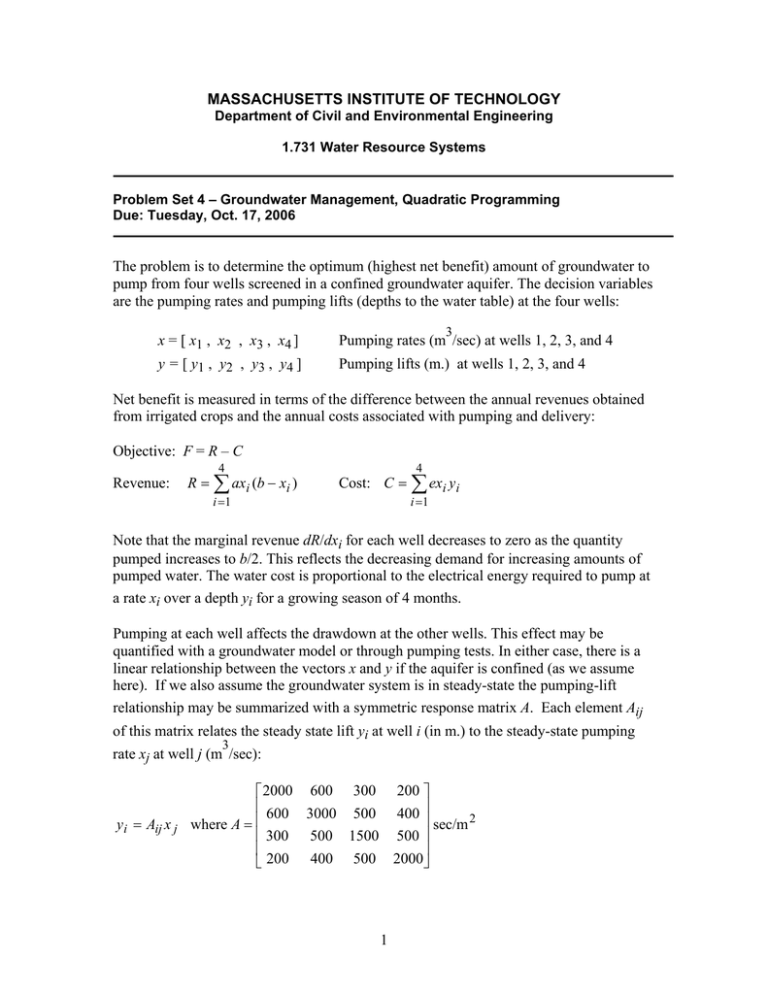
MASSACHUSETTS INSTITUTE OF TECHNOLOGY
Department of Civil and Environmental Engineering
1.731 Water Resource Systems
Problem Set 4 – Groundwater Management, Quadratic Programming
Due: Tuesday, Oct. 17, 2006
The problem is to determine the optimum (highest net benefit) amount of groundwater to
pump from four wells screened in a confined groundwater aquifer. The decision variables
are the pumping rates and pumping lifts (depths to the water table) at the four wells:
x = [ x1 , x2 , x3 , x4 ]
y = [ y1 , y2 , y3 , y4 ]
3
Pumping rates (m /sec) at wells 1, 2, 3, and 4
Pumping lifts (m.) at wells 1, 2, 3, and 4
Net benefit is measured in terms of the difference between the annual revenues obtained
from irrigated crops and the annual costs associated with pumping and delivery:
Objective: F = R – C
4
Revenue:
R = ∑ axi (b − xi )
i =1
4
Cost: C = ∑ exi yi
i =1
Note that the marginal revenue dR/dxi for each well decreases to zero as the quantity
pumped increases to b/2. This reflects the decreasing demand for increasing amounts of
pumped water. The water cost is proportional to the electrical energy required to pump at
a rate xi over a depth yi for a growing season of 4 months.
Pumping at each well affects the drawdown at the other wells. This effect may be
quantified with a groundwater model or through pumping tests. In either case, there is a
linear relationship between the vectors x and y if the aquifer is confined (as we assume
here). If we also assume the groundwater system is in steady-state the pumping-lift
relationship may be summarized with a symmetric response matrix A. Each element Aij
of this matrix relates the steady state lift yi at well i (in m.) to the steady-state pumping
3
rate xj at well j (m /sec):
⎡2000 600 300 200 ⎤
⎢ 600 3000 500 400 ⎥
⎥ sec/m 2
yi = Aij x j where A = ⎢
⎢ 300 500 1500 500 ⎥
⎢
⎥
⎣ 200 400 500 2000⎦
1
When the response matrix relationship is substituted in the objective function expressions
above the result is a quadratic objective. For a GAMS solution to this problem the
response matrix equation and the definitions of R and C may be included as a set of
equality constraints. Then the objective function can be written in terms of the
intermediate decision variables R and C.
Additional problem constraints are:
xi ≤
b
2
yi ≤ 30
xi ≥ 0
yi ≥ 0
for all i
Assume that:
a = 4.0 108 $/m6/sec2
3
b = .01 m /sec
In order to solve this problem, carry out the following tasks:
1). Derive the cost coefficient e, given that the price of electricity is $ 0.20 / kwhr.
2). Check to see if a local maximum for this problem is also global (i.e. is the
objective function concave?). To check this you will need to construct a Hessian
matrix and use MATLAB to test its eigenvalues for your particular set of problem
inputs.
3). Solve the problem using GAMS. If the objective function is not concave try a
few different initial feasible solutions to provide confidence that the GAMS
solution is a global maximum.
4). Evaluate the shadow prices associated with any pumping lift (yi) constraints
that are active at the GAMS solution.
Please hand in only enough information to adequately document your solution.
2