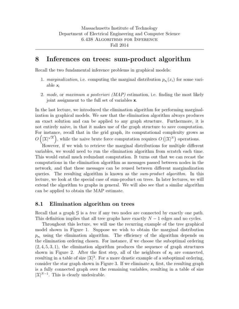
Massachusetts Institute of Technology
Department of Electrical Engineering and Computer Science
6.438 Algorithms for Inference
Fall 2014
8
Inferences on trees: sum-product algorithm
Recall the two fundamental inference problems in graphical models:
1. marginalization, i.e. computing the marginal distribution pxi (xi ) for some vari­
able xi
2. mode, or maximum a posteriori (MAP) estimation, i.e. finding the most likely
joint assignment to the full set of variables x.
In the last lecture, we introduced the elimination algorithm for performing marginal­
ization in graphical models. We saw that the elimination algorithm always produces
an exact solution and can be applied to any graph structure. Furthermore, it is
not entirely naive, in that it makes use of the graph structure to save computation.
Forr instance,
recall that in the grid graph, its computational complexity grows as
√ n
O |X| N , while the naive brute force computation requires O |X|N operations.
However, if we wish to retrieve the marginal distributions for multiple different
variables, we would need to run the elimination algorithm from scratch each time.
This would entail much redundant computation. It turns out that we can recast the
computations in the elimination algorithm as messages passed between nodes in the
network, and that these messages can be reused between different marginalization
queries. The resulting algorithm is known as the sum-product algorithm. In this
lecture, we look at the special case of sum-product on trees. In later lectures, we will
extend the algorithm to graphs in general. We will also see that a similar algorithm
can be applied to obtain the MAP estimate.
8.1
Elimination algorithm on trees
Recall that a graph G is a tree if any two nodes are connected by exactly one path.
This definition implies that all tree graphs have exactly N − 1 edges and no cycles.
Throughout this lecture, we will use the recurring example of the tree graphical
model shown in Figure 1. Suppose we wish to obtain the marginal distribution
px1 using the elimination algorithm. The efficiency of the algorithm depends on
the elimination ordering chosen. For instance, if we choose the suboptimal ordering
(2, 4, 5, 3, 1), the elimination algorithm produces the sequence of graph structures
shown in Figure 2. After the first step, all of the neighbors of x2 are connected,
resulting in a table of size |X|3 . For a more drastic example of a suboptimal ordering,
consider the star graph shown in Figure 3. If we eliminate x1 first, the resulting graph
is a fully connected graph over the remaining variables, resulting in a table of size
|X|N −1 . This is clearly undesirable.
x1
x3
x2
x4
x5
Figure 1: A tree-structured graphical model which serves as a recurring example
throughout this lecture.
x1
x1
x3
x3
x5
x4
x1
x5
x1
x3
Figure 2: The sequence of graph structures obtained from the elimination algorithm
on the graph from Figure 1 using the suboptimal ordering (2, 4, 5, 3, 1).
x2
x2
x6
x6
x3
x3
x1
x5
x4
x5
x4
Figure 3: A star-shaped graph and the resulting graph after eliminating variable x1 .
2
x1
x1
x1
x3
x2
x3
x2
x5
m4 (x2 )
m5 (x2 )
x1
x2
m4 (x2 )
m4 (x2 )
m3 (x1 )
m5 (x2 )
m2 (x1 )
m3 (x1 )
Figure 4: The sequence of graph structures and messages obtained from the elimina­
tion algorithm on the graph from Figure 1 using an optimal ordering (4, 5, 3, 2, 1).
Fortunately, for tree graphs, it is easy to find an ordering which adds no edges.
Recall that, in last lecture, we saw that starting from the edges of a graph is a
good heuristic. In the case of trees, “edges” correspond to leaf nodes, which suggests
starting from the leaves. In fact, each time we eliminate a variable, the graph remains
a tree, so we can choose an ordering by iteratively removing a leaf node. (Note that
the root node must come last in the ordering; however, it is easy to show that every
tree has at least two leaves.) In the case of the graph from Figure 1, one such ordering
is (4, 5, 3, 2, 1). The resulting graphs and messages are shown in Figure 4.
In a tree graph, the maximal cliques are exactly the edges. Therefore, by the
Hammersley-Clifford Theorem, if we assume the joint distribution is strictly positive,
we can represent it (up to normalization) as a product of potentials ψij (xi , xj ) for
each edge (i, j). However, it is often convenient to include unary potentials as well,
so we will assume a redundant representation with unary potentials φi (xi ) for each
variable xi . In other words, we assume the factorization
px (x) =
1
Z
φi (xi )
i∈V
ψij (xi , xj ).
(1)
(i,j)∈E
The messages produced in the course of the algorithm are:
m4 (x2 ) =
φ4 (x4 )ψ24 (x2 , x4 )
x4
m5 (x2 ) =
φ5 (x5 )ψ25 (x2 , x5 )
x5
m3 (x1 ) =
φ3 (x3 )ψ13 (x1 , x3 )
x3
m2 (x1 ) =
φ2 (x2 )ψ12 (x1 , x2 )m4 (x2 )m5 (x2 )
(2)
x2
Finally, we obtain the marginal distribution over x1 by multiplying the incoming
messages with its unary potential, and then marginalizing. In particular,
px1 (x1 ) ∝ φ1 (x1 )m2 (x1 )m3 (x1 ).
3
(3)
x1
x3
x2
x4
x5
Figure 5: All messages required to compute the marginals over px1 (x1 ) and px3 (x3 )
for the graph in Figure 1.
Now consider the computational complexity of this algorithm. Each of the mes­
sages produced has |X| values, and computing each value requires summing over |X|
terms. Since this must be done for each of the N − 1 edges in the graph, the total
complexity is O(N |X|2 ), i.e. linear in the graph size and quadratic in the alphabet
size.1
8.2
Sum-product algorithm on trees
Returning to Figure 1, suppose we want to compute the marginal for another variable
x3 . If we use the elimination ordering (5, 4, 2, 1, 3), the resulting messages are:
X
φ5 (x5 )ψ25 (x2 , x5 )
m5 (x2 ) =
x5
m4 (x2 ) =
X
φ4 (x4 )ψ24 (x2 , x4 )
x4
m2 (x1 ) =
X
φ2 (x2 )ψ12 (x1 , x2 )m4 (x2 )m5 (x2 )
x2
m1 (x3 ) =
X
φ1 (x1 )ψ13 (x1 , x3 )m2 (x1 )
(4)
x1
Notice that the first three messages m1 , m4 , and m2 are all strictly identical to the
corresponding messages from the previous computation. The only new message to be
computed is m1 (x3 ), as shown in Figure 5.
As this example suggests, we can obtain the marginals for every node in the graph
by computing 2(N − 1) messages, one for each direction along each edge. When
computing the message mi→j (xj ), we need the incoming messages mk→i (xi ) for its
other neighbors k ∈ N (i) \ {j}, as shown in Figure 6. (Note: the \ symbol denotes
the difference of two sets, and N (i) denotes the neighbors of node i.) Therefore, we
need to choose an ordering over messages such that the prerequisites are available at
each step. One way to do this is through the following two-step procedure.
1
Note that this analysis does not include the time for computing the products in each of the
messages. A naive implementation would, in fact, have higher computational complexity. However,
with the proper bookkeeping, we can reuse computations between messages to ensure that the total
complexity is O(N |X|2 ).
4
xj
xi
N (i) \ {j}
Figure 6: The message mi (xi ) depends on each of the incoming messages mk (xi ) for
xi ’s other neighbors N (i) \ {j}.
• Choose an arbitrary node i as the root, and generate messages going towards it
using the elimination algorithm described in Section 8.1.
• Compute the remaining messages, working outwards from the root.
We now combine these insights into the sum-product algorithm on trees. Messages
are computed in the order given above using the rule:
X
Y
mi→j (xj ) =
φi (xi )ψij (xi , xj )
mk→i (xi ).
(5)
xi
k∈N (i)\{j}
Note that, in order to disambiguate messages sent from node i, we explicitly write
mi→j (xj ) rather than simply mi (xj ). Then, the marginal for each variable is obtained
using the formula:
Y
pxi (xi ) ∝ φi (xi )
mj→i (xi ).
(6)
j∈N (i)
We note that the sum-product algorithm can also be viewed as a dynamic program­
ming algorithm for computing marginals. This view will become clearer when we
discuss hidden Markov models.
8.3
Parallel sum-product
The sum-product algorithm as described in Section 8.2 is inherently sequential: the
messages must be computed in sequence to ensure that the prerequisites are avail­
able at each step. However, the algorithm was described in terms of simple, local
operations corresponding to different variables, which suggests that it might be par­
allelizable. This intuition turns out to be correct: if the updates (6) are repeatedly
applied in parallel, it is possible to show that the messages will eventually converge
to their correct values. More precisely, letting mti (xj ) denote the messages at time
step t, we apply the following procedure:
1. Initialize all messages m0i→j (xj ) = 1 for all (i, j) ∈ E.
2. Iteratively apply the update
X
mt+1
(x
)
=
φi (xi )ψij (xi , xj )
j
i→j
xi
Y
k∈N (i)\{j}
5
t
mk→i
(xi )
(7)
Intuitively, this procedure resembles fixed point algorithms for solving equations
of the form f (x) = x. Fixed point algorithms choose some initial value x0 and then
iteratively apply the update xt+1 = f (xt ). We can view (6) not as an update rule, but
as a set of equations to be satisfied. The rule (7) can be viewed as a fixed point update
for (6). You will prove in a homework exercise that this procedure will converge to
the correct messages (6) in d iterations, where d is the diameter of the tree (i.e. the
length of the longest path).
Note that this parallel procedure entails significant overhead: each iteration of the
algorithm requires computing the messages associated with every edge. We saw in
Section 8.1 that this requires O (N |X|2 ) time. This is the price we pay for parallelism.
Parallel sum-product is unlikely to pay off in practice unless the diameter of the tree
is small. However, in a later lecture we will see that it naturally leads to loopy belief
propagation, where the update rule (7) is applied to a graph which isn’t a tree.
8.4
Efficient implementation
In our complexity analysis from Section 8.1, we swept under the rug the details of
exactly how the messages are computed. Consider the example of the star graph
shown in Figure 3, where this time we intelligently choose the center node x1 as the
root. When we compute the outgoing messages m1→j (xj ), we must first multiply
together all the incoming messages mk→1 (x1 ). Since there are N − 2 of these, the
product requires roughly |X|N computations. This must be done for each of the N −1
outgoing messages, so these products contribute approximately |X|N 2 computations
in total. This is quadratic in N , which is worse than the linear dependency
a we2 stated
earlier. More generally, for a tree graph G, these products require O (|X| i di ) time,
where di is the degree (number of neighbors) of node i.
However, in parallel sum-product, we can share computation between the different
messages by computing them simultaneously as follows:
1. Compute
⎛
⎞
Y
µti (xi ) = ⎝
mtk→i (xi )⎠ φi (xi )
(8)
k∈N (i)
2. For all j ∈ N (i), compute
mt+1
i→j (xj ) =
X ψi (xi , xj )µt (xi )
i
t
mj→i (xi )
x ∈X
(9)
i
Using this algorithm, each
a update (8) can be computed in O(|X|di ) time, so the cost
per iteration is O (|X| i di ) = O (|X|N ). Computing (9) still takes O (|X|2 ) per
node, so the overall running time is O (|X|2 N ) per iteration, or O (|X|2 N d) total.
(Recall that d is the diameter of the graph.) A similar strategy can be applied to the
sequential algorithm to achieve a running time of O(|X|2 N ).
6
MIT OpenCourseWare
http://ocw.mit.edu
6.438 Algorithms for Inference
Fall 2014
For information about citing these materials or our Terms of Use, visit: http://ocw.mit.edu/terms.