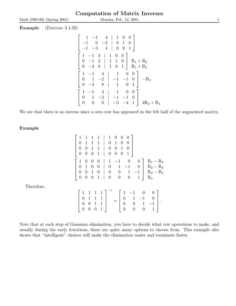
Computation of Matrix Inverses
Math 1090-001 (Spring 2001)
Example
Monday, Feb. 12, 2001
(Exercise 3.4.20)

1 −1
4 | 1
 −1
0 −2 | 0
−1 −3
4 | 0

1 −1 4 | 1 0
 0 −1 2 | 1 1
0 −4 8 | 1 0

1 −1
4 |
1
 0
1 −2 | −1
0 −4
8 |
1

1 −1
4 |
1
 0
1 −2 | −1
0
0
0 | −3
1

0 0
1 0 
0 1

0
0  R1 + R2
1
R1 + R3

0 0
−1 0  −R2
0 1

0 0
−1 0 
−4 1
4R2 + R3
We see that there is no inverse since a zero row has appeared in the left half of the augmented matrix.
Example

1
 0

 0
0

1
 0

 0
0
0
1
0
0
0
0
1
0

0
0 

0 
1
1
1
0
0
1
1
1
0
1
1
1
1
|
|
|
|
1
0
0
0
0
1
0
0
0
0
1
0
0
0
0
1
|
|
|
|

R1 − R2
1 −1
0
0
0
1 −1
0 
 R2 − R3
0
0
1 −1  R3 − R4
R4
0
0
0
1
Therefore,

1
 0

 0
0
1
1
0
0
1
1
1
0
−1 
1
1 −1
0
0


1 
0
1 −1
0
=
 0
1 
0
1 −1
1
0
0
0
1


.

Note that at each step of Gaussian elimination, you have to decide what row operations to make, and
usually during the early iterations, there are quite many options to choose from. This example also
shows that “intelligent” choices will make the elimination easier and terminate faster.