I
'P.
Problem Set 2
6.435 System Identification
Ali J. Azarbayejani
9 October
1991
1. Nonparametric time- and frequency-domain methods.
Ljung Problem 6G.3
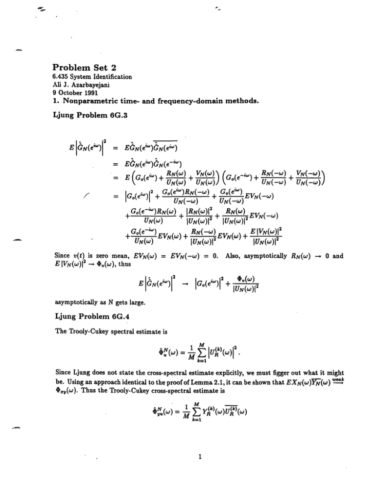
E GN(eiw)I
= EGN(ew)GN(eiw)
= EGN(eiW)GN(e-iW)
= E (Go(eiw) +
K1
f.RN(W)
NW_)V-)
N VN()\f
(G (G +
) + RN(-W)
VN(-W)
UN=(w) U(W)
UN(-W)
2+ G(e')RN(-w) G(e
Go(eiw)1
~
IC(e
UN(-W)
+ N -
)
N(
=
G,(e-"')RN(w)+ IRN(w)2
IUN(W)I
UN(w)
+ G(e-"w) EVN(
+ RN(-)
)
' ) E VN
(
IUN(W)
UN(W)EVN
Since v(t) is zero mean, EVN(W) = EVN(-w)
2 E IVN(W)I
+ RN(w)
+ RN--
= 0.
E
lGN(ei)
EV( )
,,
EVN(-w)
2
2
UN(W)1
EVN(w)I
Also, asymptotically
.v(w),thus
UN(-w)
RN()
-*
0 and
IGo(ei) I12 + ()
-*
asymptotically as N gets large.
Ljung Problem 6G.4
The Trooly-Cukeyspectral estimate is
N(W) = 1 Z
k=l
2
1U)(W)1
N
=
()
Since Ljung does not state the cross-spectral estimate explicitly, we must figgerout what it might
be. Usingan approach identical to the proof of Lemma 2.1, it can be shown that EXN(W)YN(W) '
,,(w). Thus the Trooly-Cukeycross-spectral estimate is
M
1
1y(k) )
k=1
-
1
(k)
ir
Equation (6.70) is
GN(ei)
=
1
M
Ei |U(k)(Ll2
k=l
k=1
k=l
~Nk=(w)
Ljung Problem 6E.1
For the impulse response method, we took
(t) = y(t)/a
for t = 1,..., N. An estimate for Go(ei' ) might be the Fourier transform of this estimated impulse
response:
N
G0(e"')
(t)e-iwk
=
k=l
Ek=L y(k)e-wk
v/YN(w)
VUN()
which is the ETFE after cancelling the common constant.
Ljung Problem 6E.2
Clearly, u(t) and y(t) are highly correlated, in fact they are scaled versions of one another and
UN(W)= -KYN(w).
Thus,
GN(e)
= -1/K.
The reason Lemma 6.1 does not apply here is because the feedback causes u(t) to be highly correlated with v(t). In fact,
,(t,
-K
1+ KG0 v(t)
2
i:
which implies that Euv i a nonzero function of Ev 2 . Lemma 6.1 requires uncorrelated {u(t)} and
{v(t)}.
Ljung Problem 6E.3
Take a slightly more general case. Let wk, k = 1,..., M be independent random variables with
mean m and variancesE(wk - m) 2 = Ak. Now,for
M
W= E akWk
k=l
we wish to find {ak} to satisfy (a) Ew = m, where I have changed the condition appropriately for
my slightly more general case. Since
M
E akEk
Ew =
k=l
M
= MEak
k=l
the constraint imposed by (a) is that the coefficientssum to 1:
M
Eak = 1.
k=1
Now we must consider (b), minimize E(w - m) 2 . First,
E(w - m)2
= E(
akk
= E ((
=
Z
+ m2
- 2m Eakwk
akwk
aEw
k
m)
-
+2
k
, aja
ak(Ak + m2)- 2m
2
Ewjwk -2m E ak Ewk+m2
`j
'
+
m2
k
k
where the constraint (a) has been enforced to obtain the second term of the last equality.
Since m is constant, minimizing Ek ak(Ak + m 2 ) will result in the desired minimization. Thus we
have a constrained minimization problem and can employ a Lagrange multiplier method. In this
method we would like to minimize
M
M
Q= E
k=l
a(Ak + m2) +
3
( a
k=l
-
1)
I=
The minimum can be found by where the partial derivatives w.r.t ak and p are zero. Thus,
Oak= 2ak(Ak -! n 2) +
Oak
Q
M
=E
ok -1
= 0
=0
k=l
must be satisfied. These are M + 1 independent linear equations in the unknowns {ak} and I,
hence there is a unique solution. Considering that
2
2
2a
1 j(Aj + m ) = 2ak(Ak + m )
must be satisfied for all j, k, the solution must be of the form ak = Ck/(Ak + m 2 ). The first M
partial derivativesgive ck = -p/2. Thus, from the last partial derivative,
-2
1/(Ak + m2 )
=Ek
resulting in
1
k 1/(Ak + m 2)
Ck =
Now, defining the inverse mean square as 7k = 1/(Mk + m2 ) and the sum of inverse mean squares
as SM = EkM=1 k, we have
77k
SM
For the special case m = 1, r/k = 1/(Xk + 1)The minimal variance of w, call it A is
1
2
k
1 - m 2 SM
SM
Application of this technology: Ljung equation (6.69) gives an estimate of w = GN(e i ) as the
weighted sum of independent measurements, where ak = 1/M for all k. Since the sum of alphas is
unity, the mean of the estimate is the same as the means of the measurements (assuming they all
have the same mean), but this simple set of alphas does not guarantee the minimum variance on
the estimate.
Ljung equation (6.70) again estimates GN(ei)
with
as a weighted sum of measurements, but this time
'1k)
E GR (e
Ot k1 E
w
i )
2
- Go(eiw)
2
()-
. (k)
Ek l/E CR (ei)
4
-
G.(eiw)
IU)(W)I|/'V(W)
-
-
kIU)V
(12 /t
_
IUj(k)(W)/2
Ek
(W)1|
|IUR
This estimate of the transfer function is minimum variance based on the estimates of variance for the
ETFE, which come from a finite sample of data. As R gets large, this estimate will asymptotically
have the minimum variance.
Ljung Problem 6T.2
EISNI2
N
N
E
=
aEtasv(t)v(s)
N
<
N2E
N
E
t=l s=l
lata, I (t)v(s)
N N
E R,(t - s)
N2 E
C
N t-I
N2
E
t=l r=t-N
N
2
N2 E
R,(r)
( )-
t-N-I
R.(r)-
r=--oo00
t=l
r=t
R()
\
Now, consider
N t-N
E
E
t=l r=-o
N t-N
< E
R(r)
t=l r=-oo
-N
NR,,(T·) l
-
N IR,(r)l +
r=-00oo
0
7=-00
E
r=-N+l
I IR.(r)l.
Similarly,
o
EE R()
t=l r=t
I
-1
-N
N
-r.
r=-N+1 t=l
r=-oo t=l
_<
I
IRv(r)I+
00
<
5
r=l
r IR(r)l
IrlIRv(r)I
,or
Thus,
E ISNI2
C'2 (Nt.(O) + N(2C3 ))
N
C,2(.(0O)+ 2C3 )
N
where
C2
N
00
C3 > E IrRv(r)l
-00
In relation to Lemma 6.1, relate at to e-'t,
and C1 to unity. Then, VN(w) = viSN
and
EIVN(w) 2 = NEISNI 2
< NC 2 /N = C2
= i,(O) + 2C3
with C 3 defined above. This is a somewhat weaker result than in Lemma 6.2 where it is shown that
the variance of the noise transform approaches the spectrum asymptotically for all values of w.
The technical assumption on the correlation function is not terribly restrictive because typical noise
correlations drop off rapidly. For example, a white noise satisfies the criterion and any noise with
a finite length correlation function satisfies the criterion.
2. Hum.
We have
y = Gu + v
U = U* +
V= V + W
where u* and v* are the uncorrupted input and noise processes, respectively, and w is a 60Hz hum.
By assuming that u and v have discrete frequency profiles that have no common frequency except
that of w, we can be assured that u*, v*, and w are uncorrelated.
Thus,
Vu(W)
= u() +$u'.(W)
+ Ae(w)+~w(w)
o
o
_- () +w()
(the cross terms are zero) and
U() = ,.,-U.(w)
+ ,.,(w)+t.(W) +t(w)
o
=
o
.(w)
6
o
By transforming Ey(t)u(t
-
),
we get
Dyu(W) =
C(eiW)u(w) + -vtU(w)
Thus,
G(eIw)
=
G(ew)
+tu()
' )
G(e iw
+
()
=t.(W) + w(w)
The estimate is biased. The decision to use this approach is questionable and warrants
further
review.
3. Properties and smoothing of ETFEs.
(a) Generate data.
Ten values of N were used for generating data (M=10). For k = 1,.. ., M I used Nk = 10k2
. Thus
{Nk)} = {10, 40, 90, 160,250,360,490,640,810,
1000}.
For each value of Nk, forty simulations were run (P=40). This is done with the following MATLAB
script for the ETFE estimates in part (b). A similar script was used to generate estimates using
SPA in part (c).
X
6.435 Problem Set 2
X Problem
3:
. This is the actual system for Problem 3.
a =
[1i;
b =
C[0 1];
c = [1 0.5];
d = [1 -0.2];
f =
[1-0.6];
THueto_y
= mktheta(a,b,c,d,f);
X This is for M=10 different data lengths
H = 10;
for k=l:M;
k,
...this generates the input sequence
N = 10*k^2,
Narray(k)
= N;
7
'!-
for j=l:N;
uj
= 0;
for i1:4;
u-j = U.j
end
+ cos(pi*i*j/2);
u(j) uj;
end
X ...and this generates the noise sequence.
rand('normal');
X This here simulates and estimates several times for this N
P - 40;
for
j
1:P;
e = rand(N,1);
y = idsim([u'
e,TH.ueto_y);
Gest = etfe(Ey u']);
g.pi_2(j) = Gest(65,2);
gpi(j) = G.est(129,2);
end
mx(k) = mean(gpi_2);
my(k) = mean(gpi);
varpi_2(k) = mean(diag(gpi2'*g.pi_2))- (mean(gpi_2))^2;
corr(k) = mean(diag(gpi.2'*g_pi)) - mean(gpi_2)*mean(gpi);
end
plot(Narray,varpi2);
xlabel('number
of steps, N');
ylabel('Variance at PI/2');
text(0.3,0.8,'M=10
text(O.3,0.75,'P=40
values of N','sc');
runs at each N','sc');
text(0.3,0.7,'ETFE ethod','sc');
meta graph3bvar;
pause
plot(Narray,corr);
xlabel('number
of steps, N');
ylabel('Correlationbetween PI/2 and PI');
text(0.3,0.5,'M=10
text(0.3,0.45,'P=40
values of N','sc');
runs at each N','sc');
text(0.3,0.4,'ETFE ethod','sc');
meta graph3bcorr;
(b) ETFE estimates of G.
The above MATLAB script generates ETFE estimates. At each value of Nk, the mean and variance
i ' 2) is computed
of GNk(e
from the forty data runs at that Nk. Also, the correlation between
8
10;e-
nt _1
.
--
-I
MIlU
0.1
.
.
.
.
.
.
.
.
·
values
P40 nms at eah N
ETFEMedod
0.08
U
0.06
*1
0.04
0.02
I
l
100
0
200
300
400
500
600
700
800
900
1000
number of steps, N
Figure 1: ETFE estimate of variance versus data length (P3b).
GN(e i /
2)
and (Nk(e
i
) is also computed and collected for each value of Nk.
The results are shown in Figures 1 and 2 and do confirm the theoretical properties of ETFE. Both
should asymptotically decrease, the variance to a constant number and the correlation to zero, as
described in Ljung Chapter 6.
(c) Spectral analysis.
The results are shown in Figures 3 and 4. The differences in my plots are not very marked. Both
plots exhibit the same behavior, qualitatively and, to a large extent, quantitatively.
I could comment on the tradeoff between window length and data length, but I did not include this
tradeoff in my simulations. In general, however, long windows will improve the variance but at the
expense of introducing a bias, because the windowed frequencies will have some variance among
them. For short data sequences, a long window might be the only way of achieving a low-variance
estimate. My data shows, however, that with a data length over 500 samples, a window of 1 is as
good as a window of 20. Thus for long data sequences, the window should be kept small to avoid
biasing the estimate.
4. Nonparametric identification in feedback loop.
(a) Generate data.
We start with
y = Gu + v
9
Jo!-
x10-3
I
W.
IIt
1
number of steps, N
Figure 2: ETFE estimate of correlation versus data length (P3b).
I
If
0
100
200
300
400
500
600
700
800
900
--
I000
numberof steps, N
Figure 3: Spectral estimate of variance versus data length (P3c).
10
as
!
x10-3
6:
rC
g
I
0
A:
0
200
100
300
400
500
700
600
800
900
1000
numberof steps,N
Figure 4: Spectral estimate of correlation versus data length (P3c).
v = He
u = r-Ky
G=
q-1
1- 0.5q -1
K = 0.5
H-
1 - 0.5q- 1
q
1 - 0.2q - 1
lO
After algebraic manipulation, we have
1 - 0.25q-2
Y
Y q r + 1 - 0.2q -1 e
The above system is used to generate y(t) from white sequences r(t) and e(t). Computationally,
the input u(t) is computed from the sequences r(t) and y(t). In a real experiment, u and y are
available directly. The MATLAB script is
I This is the closed loop system with input r and noise e
a = [1];
b = [0 1];
c = [1 0 -0.25];
d = E1 -0.2];
THgocl = mktheta(a,b,c,d);
X
This
is
a simulation to generate y; (u is then computed)
11
-(·
rand( 'normal');
e = rand(1000,1);
r = rand(1000,1);
y = idsim([r
e],THgcl);
u = r - 0.5*y;
(b) Estimate G, estimate ON
The correlation method for estimating the transfer function and the noise spectrum is implemented
in the MATLAB function spa. The associated formulas are (6.51) and (6.78) in Ljung. The
MATLABscript follows,the actual versus estimated transfer function is shown in Figure 5 and the
actual versus estimated noise spectrum is shown in Figure 6.
Y This is the open-loop system G with input u and output y
a = i -0.5];
b = [0 1;
c = 0;
THg = mktheta(a,b,c);
G_g = trf(THg);
'. This is the noise generator with input e and output v
a = [1 -0.2];
b = [i 0.5];
c = 0;
THh = mktheta(a,b,c);
Gh= trf(THh);
NSPvact(1,:)
= [100 0];
for k=2:length(G_h)
NSPvact(k,:) = [Gh(k,1) Gh(k,2)2];
end
%This is the spectral estimate (based on correlation)
X
the noise spectrum estimate for the data.
[Ggest NSPgest] = spa([y ul);
bodeplot( [Gg Ggest]);
' , 'sc');
text(0.2,0.85,'G,Gest for y=Gu+He,u=r-Ky
meta graph4_1;
X This is a plot of the spectrum.
bodeplot( [NSPvact NSPgest]);
text(0.2,0.85,'NSP,NSP_est for y=Gu+He,u=r-Ky','sc');
meta graph4_2;
.-
(c) Theoretical explanation.
12
and
~%..
101
AMPLITUDE PLOT, input # 1
G,G_est for y=Gu+He,u--r-Ky
100
10-1
10-2
i11· i
{
{ {ii...
100
10-1
i
101
fquacy
frequency
Figure 5: Spectral analysis vs. actual plant in feedback loop (P4b).
SPECTRUM
frequency
Figure 6: Spectral analysis vs. actual plant in feedback loop (P4b).
13
One should not expect the correlation method to work very well because the estimate is only
unbiased if the input and the noise are uncorrelated, which is not the case for our feedback loop.
The noise actual noise spectrum, as shown in Figure 6, has a relatively high gain at DC and falls
off at high frequency. Thus, we should expect a good ransfer function estimate and good noise
spectrum estimate only at high frequency, which we see is the case.
To see the details of the feedback system, consider
y = Gu + He
Taking the expectation with respect to u yields
Ryu(r) = Ey(t)u(t- r)
=
g(k)Eu(t- k)u(t - r) + E h(k)Ee(t- k)u(t - r)
k
=
k
, g(k)Ru(r- k)+ E h(k)Ru(r - k)
Ick~
k
Fourier transforming yields
,yU(w)= G(eiw)$u(w) + H(eiw)c.u(w)
Similarly, starting with
u = r- Ky= r- KGu- KHe
and taking the expectation with respect to e yields
Rue(r) = Re()-K Eg(k)Ru,(r- k)-KEh(k)R(r
0
k
k
which transforms to
u(w) = -KG(eiw)iu(w) - KH(ei)*e(w)
or
,U(w) = -KG(eiw)u.(w)
- KH(eti)*e(w)
In abbreviated notation,
+ H -KIW
= G
1+KG
Thus the spectral estimate will yield
=
+ -K IHI2
(1 + K'?)*u
G+
(1+ KG)u
and the estimate is clearly biased.
14
-
k)