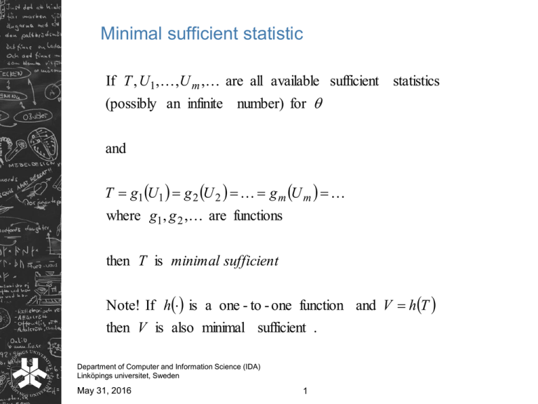
Minimal sufficient statistic
If T , U1 , , U m , are all available sufficient statistics
(possibly an infinite number) for 
and
T  g1 U1   g 2 U 2     g m U m   
where g1 , g 2 , are functions
then T is minimal sufficient
Note! If h is a one - to - one function and V  hT 
then V is also minimal sufficient .
Department of Computer and Information Science (IDA)
Linköpings universitet, Sweden
May 31, 2016
1
A statistic defines a partition of the sample space of (X1, … , Xn )
into classes satisfying T(x1, … , xn ) = t for different values of t.
If such a partition puts the sample x = (x1, … , xn ) and
y = (y1, … , yn ) into the same class if and only if
L ; x 
does not depend on 
L ; y 
then T is minimal sufficient for 
Department of Computer and Information Science (IDA)
Linköpings universitet, Sweden
May 31, 2016
2
Example
Assume again x   x1 ,  , xn  is a sample from Exp 
n
Let T  X 1 ,  , X n    X i and let T  x1 ,  , xn   t  T  y1 ,  , yn 
i 1
i.e. y   y1 ,  , yn  belongs to the same class as x
L  ; x    e
i1 xi    n e   1T  x1 ,, xn 
L  ; y    e
i1 yi    n e   1T  y1 ,, yn 
1
n 
1
n 
n
n
L  ; x   e
  1 T  x1 ,, xn T  y1 ,, y n 

  n   1T  y ,, y   e

1
n
L  ; y   e
 n   1T  x1 ,, xn 
e
  1 t t 
 1 not depending on 
 T is minimal sufficient for 
Department of Computer and Information Science (IDA)
Linköpings universitet, Sweden
May 31, 2016
3
Rao-Blackwell theorem
Let x1 ,  , xn be a random sample from a distributi on with
p.d.f f  x; 
Let T be a sufficient statistic for  and ˆ an unbiased
point estimator of 
 
Let ˆT  E ˆ T
Then
1) ˆT is a function of T alone
2) E ˆ  
 
3) Var ˆ   Var ˆ 
T
T
Department of Computer and Information Science (IDA)
Linköpings universitet, Sweden
May 31, 2016
4
The Exponential family of distributions

A random variable X belongs to the (k-parameter) exponential
family of probability distributions if the p.d.f. of X can be
written
A 1 ,, k B j  x C  x  D 1 ,, k 

j 1 j
f x;1, , k   e
k
where
A1, , Ak and D are functions of 1, ,  k alone
B1, , Bk and C are functions of x alone

What about



N(,  2 ) ?
Po( ) ?
U(0, ) ?
Department of Computer and Information Science (IDA)
Linköpings universitet, Sweden
May 31, 2016
5

For a random sample x = (x1, … , xn ) from a distribution
belonging to the exponential family
n
L1 , ,  k ; x    e
 j1 A j 1 ,, k B j  xi C  xi  D 1 ,, k 
k

i 1
e
i1  j1 A j 1 ,, k B j  xi C  xi  D 1 ,, k  
e
 j1 A j 1 ,, k  i1 B j  xi    i1C  xi  nD 1 ,, k 
e
 j1 A j 1 ,, k  i1 B j  xi    nD 1 ,, k 
n
k
k
k
n
n

n

C x 
 e i1 i 
n
 K1 in1 B1 xi , , in1 Bk  xi ;1 , ,  k  K 2  x1 , , xn 
 T  in1 B1  xi , , in1 Bk  xi  is sufficient for 1 , ,  k
In addition T is minimal sufficient (Lemma 2.5)
Department of Computer and Information Science (IDA)
Linköpings universitet, Sweden
May 31, 2016
6

Exponential family written on the canonical form:
Let 1  A1 1 , ,  k  , , k  Ak 1, ,  k 
the so - called natural or canonical parameters

k
 B  x C  x  D* 1 ,,k 

j 1 j j
f x; 1 , , k   e
where D* 1, , k   D1 , ,  k 
Department of Computer and Information Science (IDA)
Linköpings universitet, Sweden
May 31, 2016
7
Completeness



Let x1, … , xn be a random sample from a distribution with
p.d.f. f (x; )and T = T (x1, … , xn ) a statistic
Then T is complete for  if whenever hT (T ) is a function of T
such that E[hT (T )] = 0 for all values of  then
Pr(hT (T )  0) = 1
Important lemmas from this definition:



Lemma 2.6: If T is a complete sufficient statistic for  and h (T )
is a function of T such that E[h (T ) ] =  , then h is unique (there is
at most one such function)
Lemma 2.7: If there exists a Minimum Variance Unbiased
Estimator (MVUE) for  and h (T ) is an unbiased estimator for  ,
where T is a complete minimal sufficient statistic for  , then h (T
) is MVUE
Lemma 2.8: If a sample is from a distribution belonging to the
exponential family, then (B1(xi ) , … , Bk(xi ) ) is complete and
minimal sufficient for 1 , … , k
Department of Computer and Information Science (IDA)
Linköpings universitet, Sweden
May 31, 2016
8
Maximum-Likelihood estimation
Consider as usual a random sample x = x1, … , xn from a distribution
with p.d.f. f (x;  ) (and c.d.f. F(x;  ) )
The maximum likelihood point estimator of  is the value of  that
maximizes L( ; x ) or equivalently maximizes l( ; x )
Useful notation:
ˆML  arg max L ; x 

With a k-dimensional parameter:
θˆML  arg max Lθ; x 
θ
Department of Computer and Information Science (IDA)
Linköpings universitet, Sweden
May 31, 2016
9
Complete sample case:
If all sample values are explicitly known, then
ˆML
 n

n

 arg max  f xi ;   arg max  ln f xi ; 


 i 1

 i 1

Censored data case:
If some ( say nc ) of the sample values are censored , e.g. xi < k1 or xi >
k2 , then
ˆML
 n  nc


nc ,l
nc ,u 
 arg max   f  xi ;   Pr  X  k1   Pr  X  k 2  

 i 1


where
nc,l  Number of values known only as being below k1 (left - censored)
nc,u  Number of values known only as being above k 2 (right - censored)
nc,l  nc,u  nc
Department of Computer and Information Science (IDA)
Linköpings universitet, Sweden
May 31, 2016
10
When the sample comes from a continuous distribution the censored data
case can be written
ˆML
 n  nc


nc ,l
nc ,u 


 arg max   f xi ;   F k1 ;   1  F k 2 ;  

 i 1


In the case the distribution is discrete the use of F is also possible: If k1
and k2 are values that can be attained by the random variables then we
may write
ˆ
ML
 n  nc


 arg max   f  xi ;   F k1  ;

 i 1

 
  1  F k
nc ,l
 
2
;

nc ,u



where
k1  is a value  k1 but  the attainable value closest t o the left of k1
k2  is a value  k2 but  the attainable value closest t o the right of k2
Department of Computer and Information Science (IDA)
Linköpings universitet, Sweden
May 31, 2016
11
Example
x   x1 ,  , xn  random sample (R.S.) from
the Rayleigh distributi on with p.d.f.
f  x;  
x

ex
2
2
, x  0 ,  0
xi2 
 x  x 2 2  n 
l  ; x    ln  e
    ln xi  ln    
 

 i 1 
i 1
n
1 n 2
  ln xi  n ln    xi
n

i 1
l
n 1
  2

 
i 1
l
n 1
x
;

0

 2


 
i 1
n
2
i
1 n 2
   xi (case   0 excluded)
n i 1
Department of Computer and Information Science (IDA)
Linköpings universitet, Sweden
May 31, 2016
12
n
x
i 1
2
i

 2l
n
2 n 2
 2l
 2  3  xi  2
2

  i 1


n3

2



  xi2 
 i 1 
1 n 2
1 n 2
ˆ
    xi defines a (local) maximum   ML   xi
n i 1
n i 1
n
1
n i 1
   xi2


  xi2 
 i 1 
2
2n 3
n
Department of Computer and Information Science (IDA)
Linköpings universitet, Sweden
May 31, 2016
13
n
n3


  xi2 
 i 1 
n
2
0
Example
x  4,3,5,3, "  5" R.S. from the
Poisson distributi on with p.d.f. (mass function)
f  x;   
x
e 
x!
One of the sample values is right - censored : x5  5
 ˆML
 4


 arg min   f  xi ;   Pr  X  5 


 i 1

 4


 arg min   ln f  xi ;   ln Pr  X  5 


 i 1

Department of Computer and Information Science (IDA)
Linköpings universitet, Sweden
May 31, 2016
14
 4  xi   
   y  y 
 arg min   ln 
e    ln   e  

 i 1  xi !

 y 6 y!

y
5
 4




 
 arg min   xi ln   ln xi !   ln 1   e 

 i 1

 y 0 y!

Too complicated to find an analytical solutions.
Solve by a numerical routine!
Department of Computer and Information Science (IDA)
Linköpings universitet, Sweden
May 31, 2016
15
Exponential family distributions:
Use the canonical form (natural parameterization):
*




 

B
x

C
x

D
 j j
k
f x;   e j1
Let
n
T j X    B j X i  ,
j  1, , k
i 1
and assume T j  x   t j ,
j  1, , k
Then the maximum likelihood estimators (MLEs) of 1, … , k are found
by solving the system of equations


E T j X   t j ,
j  1, , k
Department of Computer and Information Science (IDA)
Linköpings universitet, Sweden
May 31, 2016
16
Example
x  x1 ,  , xn  R.S. from the Poisson distributi on
f x;   
x
e

e
x ln   ln x! 
x!
 f  x;   , i.e.   ln 
x  ln x! e
e
n
 Bx   x  T  X    X i
i 1
 MLE is found by solving
n
n
 n
 n
E   X i    xi   E  X i    xi
i 1
i 1
 i 1  i 1
Department of Computer and Information Science (IDA)
Linköpings universitet, Sweden
May 31, 2016
17


E  X i    x  f  x;     x  e


x 0
e 
x
x 1
x  ln x! e
 x
e
x!
e


x 1

 y  x 1  e


y 0
e 
 x

x  1!
e 
 y
y!
e
 e
n
n
n
i 1
i 1
i 1
e


x 0
e

e


 e 1  e
  e   xi  ne   xi  e  x
Department of Computer and Information Science (IDA)
Linköpings universitet, Sweden
May 31, 2016
18
e 
 x 1
x!
 x  1! e
x 1
 ˆML  ln x

e 
x
 x
 e
e
 e


Computational aspects
When the MLEs can be found by evaluating
l
0
θ
numerical routines for solving the generic equation g( ) = 0 can be used.
•
Newton-Raphson method
Fisher’s method of scoring (makes use of the fact that under regularity
conditions:
•
  l θ; x    l θ; x   
  2l θ; x  



  
E
  E 
 θi  j 
  i    j  





)
This is the multidimensional analogue of Lemma 2.1 ( see page 17)
Department of Computer and Information Science (IDA)
Linköpings universitet, Sweden
May 31, 2016
19
When the MLEs cannot be found the above way other numerical routines
must be used:
•
Simplex method
•
EM-algorithm
For description of the numerical routines see textbook.
Maximum Likelihood estimation comes into natural use not for handling
the standard case, i.e. a complete random sample from a distribution
within the exponential family , but for finding estimators in more nonstandard and complex situations.
Department of Computer and Information Science (IDA)
Linköpings universitet, Sweden
May 31, 2016
20
Example
x1 ,  , xn R.S. from U a, b 
b  a 1 a  x  b
 f  x; a, b   
otherwise
 0
b  a  n a  x1  x2     xn   b
 La, b; x   
otherwise
 0
 La, b; x  is as largest () when b  a (degenerat ed case).
No local maxima or minima exist.
Department of Computer and Information Science (IDA)
Linköpings universitet, Sweden
May 31, 2016
21
 La, b; x  is maximized with respect t o the sample
when b  a is as small as possible
 Choose the smallest possible approximat ion of b and the
largest possible approximat ion of a from the values in the sample
 bˆML  xn  and aˆ ML  x1
Department of Computer and Information Science (IDA)
Linköpings universitet, Sweden
May 31, 2016
22
Properties of MLEs
Invariance:
If θ and φ represent two alternativ e parameteri zations
and φ is a one - to - one function of θ : φ  g θ   θ  hφ,
then if θˆ is the MLE of θ  g θˆ is the MLE of φ

Consistency:
Under some weak regularity conditions all MLEs are consistent
Department of Computer and Information Science (IDA)
Linköpings universitet, Sweden
May 31, 2016
23
Efficiency:
Under the usual regularity conditions:

ˆML is asymptotic ally distribute d as N  , I1

(Asymptotically efficient and normally distributed)
Sufficiency:
ˆML unique MLE for   ˆML is a function of the
minimal sufficient statistic for 
Department of Computer and Information Science (IDA)
Linköpings universitet, Sweden
May 31, 2016
24
Example

x R.S. from N  ,  2


2

x 

1
f x;  ,  2 

2 2
e
x 2 2 x   2
ln  ln 2 
2 2
e
2


2 2
 x 
1
1
 ln  2  ln 2 
2
2 2
e 2
2

1
1
2
2
 2  x  2  x  ln 2  ln   2

2
2
2
 e 2
1
2
2

n
n
2 n
 2  x  2  xi  ln 2  ln   2

2
2
2
 e 2
1

2
i
 L  , 2 ; x
1

 1   2 and 2  2 ; T1  X    X i2 and T2  X    X i
2

Department of Computer and Information Science (IDA)
Linköpings universitet, Sweden
May 31, 2016
25
 1
E T1  X    E X  n     n 
  22
 21
n
E T2  X    E  X i   n  n 22   2
21
 ˆ
and ˆ
are obtained by solving
  
2
i
1, ML
2
2


2 , ML
 1
22 
n 
 2    xi2
 21 41 
n
 2   xi
21
Department of Computer and Information Science (IDA)
Linköpings universitet, Sweden
May 31, 2016
26

2

 1
22 
  n 
 2 
2

41 
1


 1  21 x 2 
2

 2  21 x  n 


x

i 
2

41 
 21
 1
1
2
1
2
ˆ
  
  x    n  xi  1, ML 

2
1
2
2  x   n  xi
 21

1

2
2 n 1   xi  x 


 ˆ
2 , ML


1
 2   
 2 n 1   x  x 2
i


Department of Computer and Information Science (IDA)
Linköpings universitet, Sweden
May 31, 2016
27


x
 x 
2
1



n
x

x
 i


Invariance property 
 1 

 2  has a one - to - one relationsh ip with  
 
 2 
(as the system of relating equations has a unique solution)

2
ˆ ML

1
2ˆ
 n 1   xi  x 
2
1, ML
2
ˆ ML  ˆ ML
 ˆ2, ML  x
 
2
Note! bias ˆ ML
 0 but  0 as n  
Department of Computer and Information Science (IDA)
Linköpings universitet, Sweden
May 31, 2016
28


1
l  , ; x  
2
2

n
n
2 n
 2   xi  ln 2  ln   2
2
2

2
2

x

i
2
2
l
1
n
 2   xi  2
 

l

 2l


2
2
1
 
2

 2l
 

2 2


 
2 2
  xi 
2
2
n 2

 
2
2 2
2
1

  xi 
2
n
 
 
1
2
2
2

x


i
3
 
2
2 2
 
2 3
  xi 
Department of Computer and Information Science (IDA)
Linköpings universitet, Sweden
May 31, 2016
n
n

 2
 2l
2

x

i
2 2
29
n

n 2
   
2
2 2
2 3

l  , 2 ; x








  2l  ,  2 ; X 
n

E 


2
2






  2l  ,  2 ; x 
1
n

E 



n


0
2
2
2

2
2


 

 
 
  2l  ,  2 ; x 
1
2
n
2
2


E

n    
 n 
2 3
2 3
 2 2 


22


n
2


with
θ


,

2
22
 
 


 
 n
  2l  ,  2 ; x    2
  
I θ   E 
2
θ

  0






0 

n 
4 
2 
Department of Computer and Information Science (IDA)
Linköpings universitet, Sweden
May 31, 2016
30
 

n 2
   
2
2 3


I θ1
 I θ , 2, 2
1

 
det I θ    I θ , 2,1
 2

 n

 0

 n
 4
 I θ ,1, 2 
1
 2


n
n
I θ ,1,1 
 0


0

0

2
4
 2


0 

n 
2
 

0 

2 4 

n 

 2


ˆ

  ML 


  2  is asymptotic ally distribute d as N   2 ;  n
   
 ˆ ML 

 0



0 

2 4  

n 
i.e. the two MLEs are asymptotically uncorrelated (and by the normal
distribution independent)
Department of Computer and Information Science (IDA)
Linköpings universitet, Sweden
May 31, 2016
31
Modifications and extensions
Ancillarity and conditional sufficiency:
T  T1  X , T2  X  a minimal sufficient statistic
for θ  θ1 , θ2 
a) fT2 t  depends on θ2 but not on θ1
b) fT1 T2 t T2  t 2  depends on θ1 but not on θ2
 T2 is said to be an ancillary statsitic for θ1 and T1 is
said to be conditionally independent of θ2
Department of Computer and Information Science (IDA)
Linköpings universitet, Sweden
May 31, 2016
32
Profile likelihood:
With θ  θ1, θ2  and Lθ1, θ2 ; x  , if θˆ2.1 is the MLE of θ2
for a given val ue of θ1 then L θ1, θˆ2.1; x is called the


profile likelihood for θ1
This concept has its main use in cases where  1 contains the parameters of
“interest” and  2 contains nuisance parameters.
The same ML point estimator for  1 is obtained by maximizing the profile
likelihood as by maximizing the full likelihood function
Department of Computer and Information Science (IDA)
Linköpings universitet, Sweden
May 31, 2016
33
Marginal and conditional likelihood:
Lθ1 , θ2 ; x  is equivalent to the joint p.d.f. of the sample x , i.e.
f X  x; θ1 , θ2 
If u, v  is a partitioni ng of x then f X  x; θ1 , θ2   f X u,v; θ1 , θ2 
Now, if f X u,v; θ1 , θ2  can be factorized as f1 u; θ1   f 2 v u; θ1 , θ2 
and f 2 v u; θ1 , θ2  does not depend on θ1 , then inferences about θ1
can be based solely on f1 u; θ1 , the marginal likelihood for θ1.
If f X u,v; θ1 , θ2  can be factorized as f1 u v; θ1  f 2 v; θ1 , θ2 ,
then inferences about θ1 can be based solely on
f1 u v; θ1 , the conditiona l likelihood for θ1.
Again, these concepts have their main use in cases where  1 contains the
parameters of “interest” and  2 contains nuisance parameters.
Department of Computer and Information Science (IDA)
Linköpings universitet, Sweden
May 31, 2016
34
Penalized likelihood:
MLEs can be derived subjected to some criteria of smoothness.
In particular this is applicable when the parameter is no longer a single
value (one- or multidimensional), but a function such as an unknown
density function or a regression curve.
The penalized log-likelihood function is written
l P θ; x   l θ; x     Rθ 
where Rθ  is the penalty function and  is a fixed parameter
controllin g the influence of Rθ .
 is thus not estimated by maximizing
l P θ; x  , but can be
estimated by so - called cross - validation techniqu es (see ch. 9)
Note that x is not the ususal random sample here, but can be
a set of independen t but non - identicall y distribute d values
Department of Computer and Information Science (IDA)
Linköpings universitet, Sweden
May 31, 2016
35
Method of moments estimation (MM )
For a random variable X :
The rth population moment about the origin is
 r  E X r 
The rth population moment about the mean
(rth central moment) is

 r'  E  X  1 r

Department of Computer and Information Science (IDA)
Linköpings universitet, Sweden
May 31, 2016
36
For a random sample x   x1 ,  , xn  :
The rth sample moment about the origin is
n
mr  n 1  xir
i 1
The rth sample moment about the mean is
n
mr'  n 1   xi  x 
r
i 1
Department of Computer and Information Science (IDA)
Linköpings universitet, Sweden
May 31, 2016
37
The method of moments point estimator of  = ( 1, … ,  k ) is obtained by
solving for  1, … ,  k the systems of equations
 r  mr , r  1, , k or
 r'  mr' , r  1, , k
or
a mixture between t hese two 
Department of Computer and Information Science (IDA)
Linköpings universitet, Sweden
May 31, 2016
38
Example
x   x1 ,  , xn  R.S. from U a, b 
ab
2
Second central moment :  2'   2  E X 2   2 
First moment about the origin : 1   
 
2
2
3
3








1
a

b
y
b

a
b

a
a

b
  y2
dy 




 
ba
4
4
3b  a 
4
 3b  a   a
a
b
2
3
b  a b 2  ab  a 2   a 2  2ab  b 2
3b  a 
4
b

4b 2  4ab  4a 2 3a 2  6ab  3b 2



12
12
2
b 2  2ab  a 2 b  a 


12
12
Department of Computer and Information Science (IDA)
Linköpings universitet, Sweden
May 31, 2016
39
Solve for a, b the systems of equations
ab
x
2
b  a 2  ˆ 2  n 1 n x  x 2

i
12
i 1
2

2 x  2a 
 b  2x  a 
12
 ˆ 2  x  a   3ˆ 2
2
 x  a   3ˆ 2  a  x  3ˆ 2


a  x  3ˆ 2  b  2 x  x  3ˆ 2  x  3ˆ 2 not possible
since a  b
 aˆ MM  x  3ˆ 2  bˆMM  x  3ˆ 2
Department of Computer and Information Science (IDA)
Linköpings universitet, Sweden
May 31, 2016
40
Method of Least Squares (LS)
First principles:
Assume a sample x where the random variable Xi can be written
X i  m    i
where m  is the mean valu e (function) involving 
and  i is a random variable with zero mean and
constant variance  2
The least-squares estimator of  is the value of  that minimizes
n
2




x

m

 i
i 1
i.e.
ˆLS
 n

2
 arg min   xi  m  
 i 1


Department of Computer and Information Science (IDA)
Linköpings universitet, Sweden
May 31, 2016
41
A more general approach
Assume the sample can be written (x, z ) where xi represents the
random variable of interest (endogenous variable) and zi represent either
an auxiliary random variable (exogenous) or a given constant for sample
point i
X i  m ; zi    i


where E  i   0 , Var  i    i2 and Cov  i ,  j  cij

with  i2 , cij possibly functions of zi , z j
The least squares estimator of  is then

ˆLS  arg min εT Wε


where ε  1 , ,  n  and W is the
variance - covariance matrix of ε
Department of Computer and Information Science (IDA)
Linköpings universitet, Sweden
May 31, 2016
42

Special cases
The ordinary linear regression model:
X i   0  1 z1,i     p z p ,i   i  Zβ  ε
with W   2 I n and Z is considered to be a constant matrix
n


 βˆ LS  arg min   i2  
β
 i 1 
1 T
n
2
T




 arg min  xi   0  1 z1,i     p z p ,i   Z Z Z x
β
 i 1


The heteroscedastic regression model:
X i  Zβ  ε with W   2I n


T
1 1 T
ˆ
 β LS  Z W Z Z W 1 x
Department of Computer and Information Science (IDA)
Linköpings universitet, Sweden
May 31, 2016
43

The first-order auto-regressive model:
X t      X t 1      t
, W   2I n
Let x  x1, x2 , , xn  and z  *, x1, , xn1  , i.e. for the
first sample point (first ti me - point) z is not available
 X t     zt      t , t  2, , n
Department of Computer and Information Science (IDA)
Linköpings universitet, Sweden
May 31, 2016
44
The conditional least-squares estimator of  (given ) is
ˆCLS
 n 2 
 n

2
 arg min   i   arg min  xi      zi     
i 2 
i 2




 arg min ε T W1ε


T 
 0
0
n 1  and 0
where W1  
n 1 is the n  1 - dimensiona l
0

 n1 I n1 
0
 
vector of zeros   
0
 
Department of Computer and Information Science (IDA)
Linköpings universitet, Sweden
May 31, 2016
45