Two Random Variables
2
19
Two Random Variables
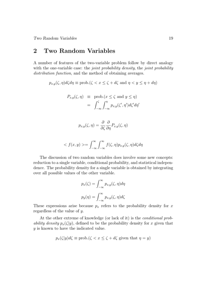
A number of features of the two-variable problem follow by direct analogy
with the one-variable case: the joint probability density, the joint probability
distribution function, and the method of obtaining averages.
px,y (ζ, η)dζdη ≡ prob.(ζ < x ≤ ζ + dζ and η < y ≤ η + dη)
Px,y (ζ, η) ≡ prob.(x ≤ ζ and y ≤ η)
ζ η
=
−∞
px,y (ζ, η) =
< f (x, y) >=
−∞
∂ ∂
Px,y (ζ, η)
∂ζ ∂η
∞ ∞
−∞
px,y (ζ , η )dζ dη −∞
f (ζ, η)px,y (ζ, η)dζdη
The discussion of two random variables does involve some new concepts:
reduction to a single variable, conditional probability, and statistical independence. The probability density for a single variable is obtained by integrating
over all possible values of the other variable.
px (ζ) =
py (η) =
∞
−∞
∞
−∞
px,y (ζ, η)dη
px,y (ζ, η)dζ
These expressions arise because px refers to the probability density for x
regardless of the value of y.
At the other extreme of knowledge (or lack of it) is the conditional probability density px (ζ|y), defined to be the probability density for x given that
y is known to have the indicated value.
px (ζ|y)dζ ≡ prob.(ζ < x ≤ ζ + dζ given that η = y)
20
Probability
Note that in the expression px (ζ|y), ζ is a variable but y is simply a parameter. px (ζ|y) has all the properties of a probability density function of
a single random variable, ζ. The following picture may be helpful in understanding the connection between the joint probability density px,y (ζ, η) and
the conditional probability density px (ζ|y).
(
(
) =
(
)
The specification that y is known restricts the possibilities to those lying on
the line η = y in the ζ – η plane. Therefore, px (ζ|y) must be proportional to
px,y (ζ, y):
px,y (ζ, y) = c px (ζ|y).
The constant of proportionality, c, can be found by integrating both sides of
the above equality over all ζ.
∞
−∞
px,y (ζ, y) dζ = py (η = y)
c
∞
−∞
px (ζ |y) dζ = c
{reduction to a single variable }
{normalization of px (ζ|y) }
1
⇒
c = py (η = y)
This result is known as Bayes’ Theorem or the fundamental law of conditional
probability:
px,y (ζ, y) = px (ζ|y)py (η = y)
Two Random Variables
21
The result can be viewed in two ways. It can be interpreted as a way of
finding the conditional density from the joint density (and the density of the
conditioning event which can be recovered from the joint density):
p(x|y) =
p(x, y)
.
p(y)
This view is illustrated in the previous figure where p(x|y) is exposed by
‘slicing through’ p(x, y). Alternatively Bayes’ theorem can be interpreted as
a way of constructing the joint density from a conditional density and the
probability of the conditioning variable:
p(x, y) = p(x|y)p(y).
This is illustrated below for the two possible choices of conditioning variable.
Here, as with store-bought bread, one can reassemble the loaf by stacking
the individual slices side by side.
22
Probability
The two random variables are said to be statistically independent (S.I.)
when their joint probability density factors into a product of the densities of
the two individual variables:
px,y (ζ, η) = px (ζ)py (η)
if x and y are S.I.
Physically, two variables are S.I. if knowledge of one gives no additional
information about the other beyond that contained in its own unconditioned
probability density:
p(x|y) =
p(x, y)
= p(x)
p(y)
if x and y are S.I.
Example: Uniform Circular Disk
Given The probability of finding an event in a two dimensional space is
uniform inside a circle of radius 1 and zero outside of the circle.
p(x, y) = 1/π x2 + y 2 ≤ 1
= 0 x2 + y 2 > 1
Problem Find p(x), p(y), and p(x|y). Are x and y S.I.?
Solution
p(x) =
∞
−∞
= 0
√1−x2
p(x, y) dy =
√
− 1−x2
1
2√
dy =
1 − x2
π
π
|x| ≤ 1
|x| > 1
Two Random Variables
23
By symmetry, the functional form for p(y) will be identical.
2
1 − y2
π
= 0
|y| ≤ 1
p(y) =
|y| > 1
It is apparent that the product of p(x) and p(y) does not equal p(x, y), so the
random variables x and y are not S.I. The conditional probability is found
from Bayes’ theorem.
p(x|y ) =
=
p(x, y)
(1/π)
{when x2 ≤ 1 − y 2 }
√
=
p(y)
(2/π) 1 − y 2
{when y 2 ≤ 1}
1
2 1 − y2
= 0
√
|x| ≤
1 − y2
elsewhere
It is not surprising that p(x|y) is a constant when one considers the following
interpretation.
24
Probability
.....................................
Example: Derivation of the Poisson Density
Given Events occurring at random alone a line X are governed by the
following two conditions:
• In the limit ∆X → 0 the probability that one and only one event occurs
between X and X + ∆X is given by r∆X, where r is a given constant
independent of X.
• The probability of an event occurring in some interval ∆X is statistically independent of events in all other portions of the line.
Problem
a) Find the probability p(n = 0; L) that no events occur in a region of
length L. Proceed by dividing L into an infinite number of S.I. intervals
and calculate the joint probability that none of the intervals contains
an event.
b) Obtain the differential equation
d
p(n; L) + rp(n; L) = rp(n − 1; L)
dL
as a recursion relation governing the p(n;L).
Two Random Variables
25
c) Show that the Poisson density
p(n; L) =
1
(rL)n e−rL
n!
is a solution of the equation. Is it unique?
Solution
a) To find p(n = 0; L) divide L into intervals each of length dL:
Consider dL so short that p(0) >> p(1) >> p(n > 1) in dL. But the
probabilities must sum to unity, p(0) + p(1) + p(2) + · · · = 1, so one can find
an approximation to p(0) which will be valid in the limit of small dL.
p(0) ≈ 1 − p(1) = 1 − r(dL)
The probability of an event in any sub-interval is S.I. of the events in
every other sub-interval, so
m=L/dL
p(n = 0; L) =
(1 − r(dL))
m=1
ln p(n = 0; L) =
ln(1 − r(dL))
m
m=L/dL
ln p(n = 0; L) ≈
−r(dL)
m=1
L
r(dL) = −rL
= −
dL
p(n = 0; L) = e−rL
26
Probability
Note that 0∞ p(n = 0; L) dL =
1 since p(n = 0; L) is not a probability density
for L, rather it is one element of a discrete probability density for n which
depends on L as a parameter.
b) Now consider the span X = 0 to X = L + ∆L to be composed of the finite
length L and an infinitesimal increment ∆L.
The two intervals are S.I. so one may decompose p(n; L + ∆L) in terms of
two mutually exclusive events.
p(n; L + ∆L) = p(n; L)p(0; ∆L) + p(n − 1; L)p(1; ∆L)
= p(n; L)(1 − r∆L) + p(n − 1; L)(r∆L)
Rearranging
p(n; L + ∆L) − p(n; L)
= rp(n − 1; L) − rp(n; L)
∆L
Passing to the limit ∆L → 0 gives
d p(n; L)
= rp(n − 1; L) − rp(n; L)
dL
Two Random Variables
27
c) To show that the Poisson density satisfies this equation, take its derivative
with respect to L and compare the result with the above expression.
p(n; L) =
1
(rL)n e−rL
n!
d
n
1
p(n; L) = r (rL)n−1 e−rL − r (rL)n e−rL
dL
n!
n!
= r
1
1
(rL)n−1 e−rL − r (rL)n e−rL
(n − 1)!
n!
= rp(n − 1; L) − rp(n; L)
This solution is unique when the differential recursion relation is supplemented by the boundary conditions
p(0; L) = e−rL
p(n; 0) = 0
n=
0.
.....................................
Extended Example: Jointly Gaussian Random Variables
Introduction The purpose of this example is to examine a particular joint
probability density and the information that can be extracted from it. We
will focus our attention on a physical example that might be encountered
in the laboratory. However, the origin of the effect is not of concern to us
now. We are interested instead in understanding and manipulating a given
probability density.
The System Consider an electronic circuit with all sources (power supplies
and signal inputs) turned off. If one looks at a given pair of terminals with
an oscilloscope, the voltage appears to be zero at low gain, but at high gain
there will be a fluctuating random voltage that might look as follows:
28
Probability
The origin of this “noise” voltage is the random thermal motion of electrons
in the components. It is referred to as “thermal noise” or “Johnson noise”
and is different from the “shot noise” associated with the quantization of
charge. This noise is still present when the sources are turned on and may
complicate the detection of a weak signal. Later in the course quantitative
expressions will be derived for the amplitude of this type of noise. For the
present, observe the following features of the voltage:
1) It has zero mean.
2) Its average magnitude |v| seems relatively well defined and excursions
too far above this magnitude are unlikely.
3) The “statistics” do not seem to change with time.
4) There is a “correlation time” τc such that over time intervals much less
than τc the signal does not change appreciably.
5) The voltages at times separated by much more than τc seem to be
statistically independent.
The noise voltage described above evolves in time and is an example of
a random process. The study of random processes is a separate field of its
own and we will not get involved with it here. Rather, we will simply note
that by evaluating the random process at two separate times we can define a
pair of random variables. For an important and frequently occurring class of
random processes the two variables thus defined will be described by a jointly
Gaussian (or bivariate Gaussian) probability density. It is this probability
density that we will examine here.
Two Random Variables
29
The Joint Probability Density
p(v1 , v2 ) =
1
v12 − 2ρv1 v2 + v22
√
]
exp[−
2σ 2 (1 − ρ2 )
2πσ 2 1 − ρ2
In the above joint probability density σ and ρ are parameters. σ is a constant, independent of time, which governs the amplitude of the variables.
ρ is a function of the time interval between the measurements, |t2 − t1 |; it
determines how strongly the two variables are correlated and is referred to
as the correlation coefficient. The magnitude of ρ is less than or equal to
one: |ρ| ≤ 1. Physically one expects that ρ will be close to one for very small
values of |t2 − t1 | and will decrease to zero for large time separations. We
will take this joint probability density as given and examine its properties.
The variables v1 and v2 appear as a quadratic form in the exponent. Thus
lines of constant probability are ellipses in the v1 , v2 plane; when ρ > 0 the
major axis will be along v1 = v2 and the minor axis will be along v1 = −v2 ;
for ρ < 0 the location of the major and minor axes is reversed. The ellipses
are long and narrow for |ρ| ∼
= 1; they become circles when ρ = 0.
30
Probability
Two Random Variables
31
Reduction to a Single Variable
Z
∞
p(v1 ) =
p(v1 , v2 ) dv2
−∞
∞
(v22 − 2ρv1 v2 + ρ2 v12 ) + (v12 − ρ2 v12 )
] dv2
2σ 2 (1 − ρ2 )
−∞
Z ∞
1
v12
(v2 − ρv1 )2
p
=
exp[− 2 ]
exp[− 2
] dv2
2σ
2σ (1 − ρ2 )
2πσ 2 1 − ρ2
−∞
|
}
√ {z
1
p
=
2πσ 2 1 − ρ2
Z
exp[−
2πσ 2 (1−ρ2 )
= √
1
2πσ 2
exp[−
v12
]
2σ 2
{a zero mean gaussian with variance σ 2 }
A similar result is found for p(v2 ).
p(v2 ) = √
1
2πσ 2
exp[−
v22
]
2σ 2
The probability densities for v1 and v2 are identical in form, so one concludes that the single
time probability densities are independent of time.
Statistical Independence
p(v1 , v2 ) = p(v1 )p(v2 )
only when ρ = 0
This implies that v1 and v2 are not statistically independent unless ρ = 0, that is, at large
time separations between t1 and t2 .
Conditional Probability
p(v2 |v1 ) =
p(v1 , v2 )
p(v1 )
= p
1
2πσ 2 (1 − ρ2 )
exp[−
(v22 − 2ρv1 v2 + v12 )
v12 (1 − ρ2 )
− 2
]
2σ 2 (1 − ρ2 )
2σ (1 − ρ2 )
1
(v2 − ρv1 )2
p
=
]
exp[− 2
2σ (1 − ρ2 )
2πσ 2 (1 − ρ2 )
This is a Gaussian with mean ρv1 and variance σ 2 (1 − ρ2 ).
32
Probability
Compare these plots of p(v2 |v1 ) with an imaginary cut of one of the plots of
p(v1 , v2 ) by a vertical plane at constant v1 . This will allow you to picture the
Two Random Variables
33
relation
p(v2 |v1 ) ∝ p(v1 , v2 ).
The exact dependence of ρ on |t2 − t1 | depends on the details of the circuit
in which the voltage is measured.
The Correlation Function The correlation function for a random process
such as the noise voltage we are discussing is defined as
R(τ ) ≡< v(t)v(t + τ ) > .
Here we have assumed that the statistics of the process do not change with
time so that the correlation function depends only on the time difference,
not the actual times themselves. In our notation then τ = t2 − t1 and
R(τ ) = R(t2 − t1 ). We can now find the correlation function in terms of the
parameters appearing in the joint probability density.
< v1 v 2 > =
=
=
∞ ∞
−∞
−∞
−∞
−∞
∞ ∞
∞
−∞
= ρ(τ )
v1 v2 p(v1 , v2 ) dv1 dv2
v1 v2 p(v2 |v1 )p(v1 ) dv1 dv2
∞
v1 p(v1 )
v2 p(v2 |v1 ) dv2
dv1
conditional mean = ρ(τ )v1
∞
−∞
−∞
v12 p(v1 ) dv1
<v 2 >=σ 2
Thus the correlation function for the random process can be written in the
simple form R(τ ) = σ 2 ρ(τ ) and the correlation coefficient ρ can be interpreted
as the normalized correlation function for the process.
In the figures presented above ρ has been displayed, for simplicity, as
positive. However for some random processes ρ may become negative, or
even oscillate, as it decays toward zero. Consider the random process that
generates the following output.
34
Probability
The frequencies which contribute to the process seem to be peaked around
500 Hz. Thus if the signal were positive at a given time one might expect
that it would be negative half a “period” later (1 ms) and, more likely than
not, positive again after a delay of 2 ms. This physically expected behavior
is reflected in the τ dependence of the correlation coefficient shown below.
One possible random process with these characteristics is the noise voltage
of an electronic circuit that is resonant near a single frequency. If the circuit
had a very high Q, the correlation function might oscillate many times before
falling away to zero.
.....................................
MIT OpenCourseWare
http://ocw.mit.edu
8.044 Statistical Physics I
Spring 2013
For information about citing these materials or our Terms of Use, visit: http://ocw.mit.edu/terms.