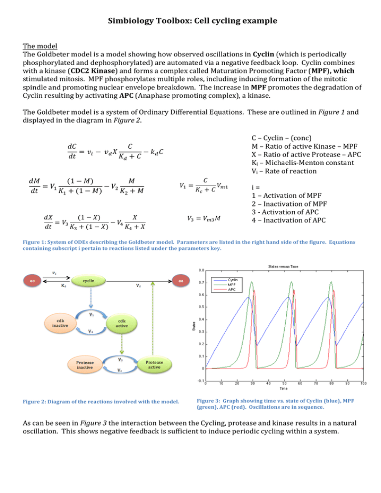
Simbiology Toolbox: Cell cycling example The model The Goldbeter model is a model showing how observed oscillations in Cyclin (which is periodically phosphorylated and dephosphorylated) are automated via a negative feedback loop. Cyclin combines with a kinase (CDC2 Kinase) and forms a complex called Maturation Promoting Factor (MPF), which stimulated mitosis. MPF phosphorylates multiple roles, including inducing formation of the mitotic spindle and promoting nuclear envelope breakdown. The increase in MPF promotes the degradation of Cyclin resulting by activating APC (Anaphase promoting complex), a kinase. The Goldbeter model is a system of Ordinary Differential Equations. These are outlined in Figure 1 and displayed in the diagram in Figure 2. C – Cyclin – (conc) 𝑑𝐶
𝐶
M – Ratio of active Kinase – MPF = 𝑣! − 𝑣! 𝑋
− 𝑘! 𝐶 X – Ratio of active Protease – APC 𝑑𝑡
𝐾! + 𝐶
Ki – Michaelis-­‐Menton constant Vi – Rate of reaction 𝐶
𝑑𝑀
(1 − 𝑀)
𝑀
𝑉! =
𝑉!! = 𝑉!
− 𝑉!
i = 𝐾! + 𝐶
𝑑𝑡
𝐾! + (1 − 𝑀)
𝐾! + 𝑀
1 – Activation of MPF 2 – Inactivation of MPF 3 -­‐ Activation of APC 𝑑𝑋
(1 − 𝑋)
𝑋
𝑉! = 𝑉!! 𝑀 4 – Inactivation of APC = 𝑉!
− 𝑉!
𝑑𝑡
𝐾! + (1 − 𝑋)
𝐾! + 𝑋
Figure 1: System of ODEs describing the Goldbeter model. Parameters are listed in the right hand side of the figure. Equations containing subscript i pertain to reactions listed under the parameters key. Figure 2: Diagram of the reactions involved with the model. Figure 3: Graph showing time vs. state of Cyclin (blue), MPF (green), APC (red). O scillations are in sequence. As can be seen in Figure 3 the interaction between the Cycling, protease and kinase results in a natural oscillation. This shows negative feedback is sufficient to induce periodic cycling within a system.
Constructing the Model: Rules vs Reactions Figure 4: Visual representation of the 'Reactions' model. This is where the model is constructed SimBiology models can be constructed with rules (systems of ODEs) and with reactions. These are then simulated/solved using SUNDIALS solvers. The GUI for both are similar, areas for editing individual rules/reactions and a table of species/constants as can be seen in Figure 2 and Figure 3. The Reactions model is constructed using the visual representation (Figure 1) and then can be edited using the dialogue (Figure 2). The Rules model is constructed using equations in the dialogue (Figure 3) and can then be visualised via the representation in Figure 4. In practise, very little is done with this particular interface. Figure 2: 'Reaction' model editor with labels. These components are found in the ‘Rules’ method with some differences. Figure 6: 'Rules' dialogue where model is constructed Figure 7: Model can be visualised here