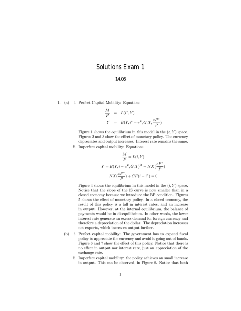
Solutions Exam 1
14.05
1. (a)
i. Perfect Capital Mobility: Equations
M
P
Y
= L(i∗ , Y )
= E(Y, i∗ − π e , G, T,
εP ∗
)
P
Figure 1 shows the equilibrium in this model in the (ε, Y ) space.
Figures 2 and 3 show the effect of monetary policy. The currency
depreciates and output increases. Interest rate remains the same.
ii. Imperfect capital mobility: Equations
M
= L(i, Y )
P
Y = E(Y, i − π e , G, T )D + N X(
N X(
εP ∗
)
P
εP ∗
) + CF (i − i∗ ) = 0
P
Figure 4 shows the equilibrium in this model in the (i, Y ) space.
Notice that the slope of the IS curve is now smaller than in a
closed economy because we introduce the BP condition. Figures
5 shows the effect of monetary policy. In a closed economy, the
result of this policy is a fall in interest rates, and an increase
in output. However, at the internal equilibrium, the balance of
payments would be in disequilibrium. In other words, the lower
interest rate generate an excess demand for foreign currency and
therefore a depreciation of the dollar. The depreciation increases
net exports, which increases output further.
(b)
i. Perfect capital mobility: The government has to expand Þscal
policy to appreciate the currency and avoid it going out of bands.
Figure 6 and 7 show the effect of this policy. Notice that there is
no effect in output nor interest rate, just an appreciation of the
exchange rate.
ii. Imperfect capital mobility: the policy achieves an small increase
in output. This can be observed, in Figure 8. Notice that both
1
LM
ε
IS
Y
Figure 1:
ε
LM 0
LM 1
ε1
ε0
IS 0
Y
Figure 2:
2
LM0
LM1
i
i*
IS1
IS0
Y
Figure 3:
i
LM 0
IS 0
Y
Figure 4:
3
i
LM0
LM1
E0
i0
*
*
i1
E1
IS1
IS0
Y
Figure 5:
ε
LM 0
ε0
ε1
IS 0
Y
Figure 6:
4
LM 0
i*
IS 1
IS 0
Y
Figure 7:
output and interest rates increase. As CF increase we need net
exports to decrease and thus the exchange rate appreciates but
less than before. The reason is that the appreciation required
to restore external equilibrium (BP=0) is smaller than under
perfect capital mobility.
(c) Notice that now NX= -b-CF. Replacing that in the IS curve we have
Y = E(Y, i − πe , G, T )D − CF (i − i∗ ) − b.
This implies that for all level of i, Y is going to be smaller, i.e. the
IS curve shifts to the left. See Figure 9.
(d) Thus both interest rate and output fall. The intervention, in which
the central bank buys domestic currency, causes the domestic currency to appreciate. The fact that the IS curve shifts to the left tells
us that output is smaller for a given price. Thus, the AD curve is also
shifting to the left and in equilibrium we have a lower price level.
(e) You are basically asked to discuss overshooting in this part. In particular, assume that the IS curve does not adjust immediately. Then
as a consequence of expansive monetary policy we have a depreciation (we know that from part 1) and a decrease in the interest rate.
See Figure 10. Notice that now we are using the fact that the IS
curve does not adjust immediately. What happens in the long run?
We know, because of long run neutrality of money, that in the long
run prices and exchange rate both increase 1 to 1 with the increase
in the quantity of money. So, there is a depreciation in the long run.
And as we just argued, there is a depreciation also in the short run.
5
i
LM
E1
E0
IS1
IS0
Y
Figure 8:
LM0
i
IS0
IS1
Y
Figure 9:
6
LM0
i
IS0
IS1
Y
Figure 10:
Which one is bigger? Do we jump to the long run value from the
beginning? No. The reason is that now i < i∗ . Thus if we jump
today to the long run value for the exchange rate then there is no
expected change on the exchange rate and capital leaves the country. But if capital is leaving the country, there is less demand for the
domestic currency and the currency depreciates. So this can’t be an
equilibrium. The same reasoning applies for a smaller devaluation in
the short run. For capital to stay here we need to compensate for
the fact that the interest rate is smaller. And according to the UIP
i = i∗ + E(úε/ε) ⇔ E(úε/ε) = i − i∗ < 0,
which implies that investors should be expecting an appreciation all
the way to the long run in order for the capital to stay. And the only
way this can happen is if the currency devaluates today more than
in the future!!!!
2. Bejamin Strong’s fears:
(a) The effect of abandoning the gold standard (Þxed exchange rate),
ßoating the exchange rate and increasing the money supply is a depreciation of the currency and an increase in output. Both effect can
be observed in Figure 11. The exchange rate increases from ε0 to ε1
and output increases from Y0 to Y1 . As in this part of the question
we are assuming small country, the interest rate remains unaffected.
(b) All the countries are identical, therefore we have to relax the small
economy assumption and consider the effect of one country’s policies
7
LM
ε
IS0
e1
e0
Y0
Y1
Y
Figure 11:
on the other. In particular, it is important to realize that if all the
countries are devaluing their currency by the same amount, then the
exchange rates, which represent the price of one currency interms of
the other, remain the same. This is equivalent to the simultaneous
devaluation case that you studied in the large economy model. Now,
to determine what happens to output we only have to realize that
the expansion obtained in part (a) has 2 components. The Þrst is the
direct effect of the increase in money supply, which increases output
along the IS. The second is the depreciation effect which shifts the IS.
In this case we have the money supply effect, but not the depreciation
effect. Therefore, the increase in output has to be smaller. The
situation is depicted in Figure 12.
(c) The hint is telling us that after the second country devalues, the
situation is going to be like in part (b): output is going to be smaller
than in part (a), but it is still going to be higher than before any
country devalued. Putting both results together we have that before
the rest of the world follows, ouput is going to increase as much as
in (a), however, after the rest of the world devalues, output is going
to fall to the level obtained in (b). In summary, the country we
are analyzing is going to have a large expansion in output followed
by small contraction. Something similaris going to happen to the
exchange rate, it will depreciate after the initial move (to the level
8
IS0
LM
ε
IS1
e0
Y0
Y2
Y1
Y
Figure 12:
ε1 ), but it will return to its original value after the rest of the world
follows (to the level ε0 ). The situation is presented in Figure 13.
(d) What is happening here is that the pattern of expansion-contraction
observed in part (c) is going to repeat indeÞnitely. Under this circumstances, both, exchange rate and output will follow a seesaw
trayectory in time. The trayectory of exchange rate is presented in
Figure 14. The trayectory of output is analogous.
(e) In this case you have to realize that all the analysis we are making
is on the side of aggregate demand. So far we have implicitly assumed that aggregate supply remains Þxed (Þx prices). Now, when
we want to analyze price ßuctuations, we have to put ourselves in a
situation in which the aggregate demand is upward sloping. Under
this assumption, the shifts in output that we have determined do
not correspond to the real equilibrium, but to shifts on the aggregate
demand. Every time the local country expands the money supply,
aggregate demands shifts outwards. Every time the rest of the world
follows, aggregate demands contracts a little, but less than it initial
expansion. Therefore, this kind of policiy keeps pushing the aggregate demand outwards indeÞnitely. It is as if aggregate demand took
two steps forward and one step back each time. At the end of the
day, prices are going to follow an increasing pattern (because prices
will lie on the AS curve). The pattern is depicted in Figure 15.
9
IS0
LM
ε
IS1
e0
e0
Y0
Y2
Y1
Y
Figure 13:
ε
e1
e0
t
Figure 14:
10
P
t
Figure 15:
3. Labor Markets
(a) Deßation will create unemployment only if nominal wages are rigid,
so they do not adjust to the fall in prices, and the real wage keeps
rising as a consequence. Assuming that the economy is initial in
its competitive equilibrium, and that nominal wages are Þx, the fall
in prices will keep increasing the real wage, and generating a gap
between the amount of labor that workers are willing to supply and
the amount of labor Þrms are willing to hire at the current real wage.
The situation is presented in Figure 16.
(b) One of the important Þndings in Nickell’s article is that countries that
follow aggresive pro-employment policies, in which there are strong
incentives for workers to go back to work and active help in reallocation by part of the government, are those which have achieved larger
reductions in the unemployment rate. The measures that Peter Hartz
is proposing are consistent with this Þndings, and to the extent that
the evidence reported in Nickell’s article is correct, we would expect
that these measures would achive a reduction in unemployment rates.
(c) A minimum wage legislation may or may not have effect in unemployment. If the minimum wage is set below the equilibrium level, it
will be no binding, and it will not induce unemployment. However,
if the minimum wage is set above the market clearing level, it will be
binding and generate unemployment. The situation is presented in
11
w/P
Ls
w0/P1
w0/P0
L1
L0
L1s
L
Figure 16:
Figure 17.
(d) If unions keep gaining strength, and they become important in the
wage bargaining process, the right kind of model to understand the
labor market is one of insiders-outsiders. We know that under the
assumptions of this model, which would be closely matched by reality, the bargaining process creates a quai-labor supply, which is
upward sloping but is located to the left of the real labor supply.
Therefore, starting from an equilibrium on the labor supply and no
unemployment, the increasing power of the unions will induce a positive amount of unemployment as depicted in Figure 18.
(e) In order to generate a procyclical wage, equilibrium on the labor
market cannot be on the labor demand. The reason is that the labor demand is downward sloping, so real wages have to fall in order
to increase output. Any of the other two models, in which equilibrium is always on the labor supply or quasi-labor supply is consistent
with the evidence. U.S. data seems more consistent with a model of
wage ßexibility and imperfect competition on the product market.
The case of ßexible wages, and imperfect competition is presented in
Figure 19.
12
w/P
U
Ls
(w/P)1
(w/P)0
Ld
L
Figure 17:
w/P
w(L)
Ls
(w/P)1
(w/P)0
Ld
U
Figure 18:
13
L
w/P
Ls
(w/P)1
(w/P)0
Ld
L
Figure 19:
14