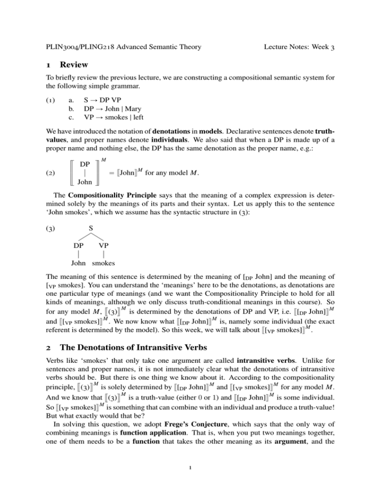
PLIN3004/PLING218 Advanced Semantic Theory
Lecture Notes: Week 3
1 Review
To briefly review the previous lecture, we are constructing a compositional semantic system for
the following simple grammar.
(1)
a.
b.
c.
S Ñ DP VP
DP Ñ John | Mary
VP Ñ smokes | left
We have introduced the notation of denotations in models. Declarative sentences denote truthvalues, and proper names denote individuals. We also said that when a DP is made up of a
proper name and nothing else, the DP has the same denotation as the proper name, e.g.:
<M
4
DP
= “ vJohnw M for any model M.
5
(2)
John
The Compositionality Principle says that the meaning of a complex expression is determined solely by the meanings of its parts and their syntax. Let us apply this to the sentence
‘John smokes’, which we assume has the syntactic structure in (3):
(3)
S
DP
VP
John smokes
The meaning of this sentence is determined by the meaning of [DP John] and the meaning of
[VP smokes]. You can understand the ‘meanings’ here to be the denotations, as denotations are
one particular type of meanings (and we want the Compositionality Principle to hold for all
kinds of meanings, although we only discuss truth-conditional meanings in this course). So
0 8M
for any model M, (3)
is determined by the denotations of DP and VP, i.e. v[DP John]w M
and v[VP smokes]w M . We now know what v[DP John]w M is, namely some individual (the exact
referent is determined by the model). So this week, we will talk about v[VP smokes]w M .
2 The Denotations of Intransitive Verbs
Verbs like ‘smokes’ that only take one argument are called intransitive verbs. Unlike for
sentences and proper names, it is not immediately clear what the denotations of intransitive
verbs should be. But there is one thing we know about it. According to the compositionality
0 8M
principle, (3) is solely determined by v[DP John]w M and v[VP smokes]w M for any model M.
0 8M
And we know that (3) is a truth-value (either 0 or 1) and v[DP John]w M is some individual.
So v[VP smokes]w M is something that can combine with an individual and produce a truth-value!
But what exactly would that be?
In solving this question, we adopt Frege’s Conjecture, which says that the only way of
combining meanings is function application. That is, when you put two meanings together,
one of them needs to be a function that takes the other meaning as its argument, and the
1
resulting meaning is the value that function returns for that argument. This is a conjecture
and there is no direct empirical evidence that this is correct, but it actually takes us very far,
as we will see throughout this course (although we will also see that we might want to have
other ‘modes of composition’ than function application). But for now, let’s assume that Frege’s
Conjecture is correct, and give an analysis to v[VP smokes]w M .
Let us first formulate the compositional rule explicitly as in (4). We call this rule the Branching Node Rule.
(4)
Branching Node Rule
4
<M
A
For any model M, 5
=
<M
4
“ vBw M pvCw M q or 5
B C
A
=
“ vCw M pvBw M q
B C
In words, if B and C are sisters in a tree, the meaning of the subtree [A B C] is either the
meaning of B applied to the meaning of C or the meaning of C applied to the meaning of
B, whichever makes sense. Usually, only one of these two possibilities makes sense. For
example, for (3), we know that v[DP John]w M is not a function but an individual. So according to (4), v[VP smokes]w M must be a function. Furthermore, it must be a function such that
v(3)w M “ v[VP smokes]w M pv[DP John]w M q. Notice that v[DP John]w M pv[VP smokes]w M q doesn’t
make sense, because v[DP John]w M is not a function.
Now, what exactly is the function v[VP smokes]w M ? It should be able to take v[DP John]w M —
0 8M
an individual—as its argument, and whenever it does, it should return (4) —a truth-value
(0 or 1)—as its output. Since v[DP John]w M can in principle be any individual in the model, it
should be able to combine with any individual in the model and for each of these individuals,
it should return a truth-value. So it’s a function from individuals to truth-values.
But what kind of truth-values should it return? If you think about the meaning of ‘John
smokes’, the denotation of this sentence should be 1 in model M if the denotation of ‘John’ in
M smokes in M, and 0 if not. So we want:
(5)
For any model M, v[DP John]w M pv[VP smokes]w M q “ 1 iff v[DP John]w M smokes in M.
Generalizing this, v[VP smokes]w M should return 1 when its input is a person who smokes in
M, and 0 when they do not smoke in M, whatever the input is.
(6)
For any model M, v[VP smokes]w M is the function that takes an individual x in M and
returns 1 iff x smokes in M.
We take this to be the denotation of [VP smokes].
As in the case of DPs, we assume that non-branching constituents like ‘[VP smokes]’ simply
inherit the meaning of its sole daughter, so we can also say that v[VP smokes]w M = vsmokesw M
for any model M. Then, we can state the denotation of the verb as follows.
(7)
For any model M, vsmokesw M is the function that takes an individual x in M and returns
1 iff x smokes in M.
The other intransitive verb in our toy grammar, ‘left’, can be given essentially the same
analysis. That is, its denotation is (8).
(8)
For any model M, vleftw M is the function that takes an individual x in M and returns 1
iff x left in M.
2
Furthermore, if you want to enrich the grammar by adding more intransitive verbs, e.g. ‘yawned’,
‘ran’, etc., it is easy to cook up the denotations of these verbs:
(9)
a.
b.
For any model M, vyawnedw M is the function that takes an individual x in M and
returns 1 iff x yawned in M.
For any model M, vranw M is the function that takes an individual x in M and returns
1 iff x ran in M.
At this point, let us state the assumption that non-branching constituents simply inherit the
denotations of their daughter constituents as a ‘compositional rule’. Although there’s no real
composition going on in such cases, you can see them as a trivial kind of composition. We call
this rule the Non-Branching Node Rule.
(10)
Non-Branching Node Rule
4 <M
A
For any model M, 5 = “ vBw M
B
To sum up, we now have the denotations for all the words and two compositional rules,
Branching Node Rule and Non-Branching Node Rule, to derive the denotations of syntactically
complex expressions, including sentences. Generally, model-theoretic semantics has these two
components, the list of words/morphemes called the Lexicon and a set of compositional rules.
For our toy grammar, the Lexicon looks like (11).
(11)
For any model M
a. vJohnw M = some individual determined by M
b. vMaryw M = some individual determined by M
c. vsmokesw M is the function that takes an individual x in M and returns 1 iff x
smokes in M
d. vleftw M is the function that takes an individual x in M and returns 1 iff x left in M
And the compositional rules are the following two.
(12)
Branching Node Rule
4
<M
A
For any model M, 5
=
“ vBw M pvCw M q or 5
B C
(13)
<M
4
A
=
“ vCw M pvBw M q
B C
Non-Branching Node Rule
4 <M
A
For any model M, 5 = “ vBw M
B
Notice that these two rules tell you how to derive the denotations of each grammatical constituent. For example, the Non-Branching Node Rule says,
v[DP John ]w M “ vJohnw M
and
v[VP smokes ]w M “ vsmokesw M
3
And Branching Node Rule says:
v[S [DP John ] [VP smokes ]]w M “ v[VP smokes ]w M pv[DP John ]w M q
“ vsmokesw M pvJohnw M q
Similarly, you can compute the meanings of all the other grammatical constituents that the
grammar produces. We will come back to this later.
In the next lecture we will enrich this semantics by adding transitive verbs likes ‘love’ to
this toy grammar.
3 Lambda-Notation for Functions
3.1
Basics
In formal semantics, it is customary to use the lambda-notation for functions, instead of
lengthy descriptions in English like ‘the function that takes an individual x and returns 1 iff
x smokes in M.’ This is largely a matter of convenience, and everything we will do in this
course could be done without the lambda-notation, but as you will soon know, it would be too
cumbersome to always use plain English to talk about functions.
In the lambda-notation, each function generally looks like:
λv : φ. α
• The symbol λ (the Greek letter ‘lambda’) has no meaning. It just signals that what follows
is a function.
• v is a variable, representing the input of the function. It’s a variable because its value varies
depending on the actual input. You can pick any variable here x, y, etc.
• φ describes what kind of input the function admits (typically in terms of v), meaning it
defines the domain of the function. Please keep in mind that φ needs to be a statement that
can be true or false. The idea is that if φ is true, the input is an appropriate kind of object
for the function to operate on, if φ is false, it is not.
• α describes the output.
It’s easier to understand this by looking at concrete examples. Here is one:
(14)
λ x : x is a natural number. x ` 5
This is a function that takes a natural number and adds 5 to it. You are probably more familiar
with the notation f pxq “ x ` 5. What’s in (14) is the same function. But the lambda-notation
is more convenient than this notation, because it is clear that you are referring to the function
itself, rather than the output value of f applied to x, which is denoted by f pxq. Also, in the
lambda-notation, you can explicitly specify the domain (i.e. ‘x is a natural number’). You can
also write (14) as (15). (Recall N is the set of natural numbers)
(15)
λ x : x P N. x ` 5
Functions like (15) where the restriction is expressed as the membership of the variable in some
set are often abbreviated to λ x P N. x ` 5. We will often use this shorthand notation.
It is important to notice that the choice of the variable x above is not important, precisely
because it is a variable. We could have chosen, say, y instead, as in (16), and meant the same
thing. So (16) and the above two functions are all the same.
4
(16)
λ y : y is a natural number. y ` 5
This is also the case in the more familiar notation. That is, f pxq “ x ` 5 and f pyq “ y ` 5
mean the same thing. Usually, we use x, y, z as variable names, but in principle they can be
any letter. It is, for example, totally legitimate to use a completely arbitrary symbol as in
K
‘λ:K
Σ P N. :Σ ` 5’, but if there’s no reason to complicate the representation, you’d better use
simple symbols for variables.
Functions need not be about mathematical operations. For instance, (17) is a legitimate
function.
(17)
λ y : y is a dog in London. y’s name
This is a function that takes any dog in London and returns its name.
Using the lambda-notation, we can re-write the denotations of the intransitive verbs as follows.
(18)
For any model M,
a. vsmokesw M “ λ x : x is an individual in M. 1 iff x smokes in M
b. vleftw M “ λ x : x is an individual in M. 1 iff x left in M
If you read published papers in formal semantics, ‘1 iff’ is often omitted, but we keep it for the
sake of explicitness. The set of all individuals in a given model (call the domain of the model)
is often written as D. Thus, these functions are more compactly written as:
(19)
3.2
For any model M,
a. vsmokesw M “ λ x P D. 1 iff x smokes in M
b. vleftw M “ λ x P D. 1 iff x left in M
Functions that return functions
Things get a bit more complicated, when you consider functions that return functions as values.
For example, we can define a function f ` that takes a natural number n, and returns a function,
which in turn take a natural number m and returns the value n ` m. As you can probably guess,
f ` represents the operation of addition. Notice that f ` p3q ‰ f ` p5q, because f ` p3q is the
function that takes a natural number and adds 3 to it, while f ` p5q is the function that takes a
natural number and adds 5 to it. In the lambda-notation, f ` can be written as (20). We use ‘[’
and ‘]’ to indicate where the function starts and ends.
(20)
f ` “ rλn P N. rλm P N. n ` mss
This function looks like it has two λ’s, but that’s not the right way of understanding it. Recall
that in the lambda-notation, each function has three parts. The first two parts are collapsed
into λn P N, which says that it takes any member n of N (which is to say that n is a natural
number) as an input. Then the output description specifies what function it turns, namely
rλm P N. n ` ms. If n “ 3, it returns rλm P N. 3 ` ms, if n “ 5, it returns rλm P N. 5 ` ms.
In the next lecture, we will analyze transitive verbs to be denoting functions that are very
similar to this.
3.3
Lambda-conversion
When a function applies to an appropriate argument, you can simplify the representation. This
process is called ‘λ-conversion’. Here is an example of vsmokesw M applied to an individual,
5
John.
vsmokesw M pJohnq “ rλ x P D. 1 iff x smokes in MspJohnq
“ 1 iff John smokes in M
We are following the standard convention that the function comes to the left of the argument and
the argument is indicated by ‘p’ and ‘q’. So things like ‘pJohnqrλ x P D. 1 iff x smokes in Ms’
and ‘pλ x P D. 1 iff x smokes in MqrJohns’ don’t make sense. These expressions are not part
of our metalanguage, and should never be used.
Here are some more examples, illustrating lambda-conversion.
(21)
a.
b.
rλ x P N. x ` 5sp12q “ 5 ` 12 “ 17
rλ x P N. x ` 5sprλ y P N. y 2 sp3qq “ rλ x P N. x ` 5sp32 q “ rλ x P N. x ` 5sp9q “
9 ` 5 “ 14
Recall that a function can return a function. Consider the following function f ´ . This
function performs subtraction.
(22)
f ´ “ rλn P N. rλm P N. n ´ mss
When one argument, say 3, is given, it returns:
f ´ p3q “ rλn P N. rλm P N. n ´ mssp3q “ rλm P N. 3 ´ ms
Here is an important convention. When two arguments follow a function, the function is applied
to the left one (= the one closer to the function) first.
f ´ p3qp2q “ rλn P N. rλm P N. n ´ mssp3qp2q “ rλm P N. 3 ´ msp2q “ 3 ´ 2 “ 1
Notice that f ´ p2qp3q “ ´1, so f ´ p3qp2q ‰ f ´ p2qp3q.
Also remember that square brackets are used to delimit functions. Notice the following
inequality:
rλn P N. rλm P N. n ´ mssp3qp2q ‰ rλn P N. rλm P N. n ´ msp3qsp2q
The left-hand side is 1, as calculated above. The right-hand side is ´1, because:
rλn P N. rλm P N. n ´ msp3qsp2q “ rλn P N. n ´ 3sp2q “ 2 ´ 3 “ ´1
Here, 3 is the argument of the inner function, and 2 is the argument of the whole function. Here
I applied the inner function to 3 first, but the order of application does not change the final
output.
rλn P N. rλm P N. n ´ msp3qsp2q “ rλm P N. 2 ´ msp3q “ 2 ´ 3 “ ´1
4 Summary and Computations
To summarize, our semantics consists of the Lexicon (23) and compositional rules (24).
(23)
For any model M
a. vJohnw M = some individual determined by M
b. vMaryw M = some individual determined by M
6
(24)
c.
d.
vsmokesw M “ λ x P D. 1 iff x smokes in M
vleftw M “ λ x P D. 1 iff x left in M
a.
Branching Node Rule
4
<M
A
For any model M, 5
b.
=
<M
4
“ vBw M pvCw M q or 5
B C
Non-Branching Node Rule
4 <M
A
For any model M, 5 = “ vBw M .
B
A
=
“ vCw M pvBw M q
B C
It is important to realize that from these, we can now compute the meanings of any grammatical constituent in the grammar. We can show this concretely by computing the meaning.
As an example, let us compute the meaning of ‘Mary left’, which has the structure in (25).
(25)
S
DP
VP
Mary left
We compute the meaning of this sentence with respect to a particular model, let’s say M3 . To
simplify, let’s assume that in M3 , ‘Mary’ refers to an individual c, and also that c left in the
situation described by M3 . That is, we will use a model M3 such that vMaryw M3 “ c and
vleftw M3 pcq “ 1. Clearly, in this model, (25) should come out true. We can prove this as
follows.
1. By the Non-Branching Node Rule, v[DP Mary]w M3 “ vMaryw M3 . Also, since vMaryw M3 “
c, we have v[DP Mary]w M3 “ c.
2. Similarly, by the Non-Branching Node Rule, v[VP left]w M3 “ vleftw M3 . Since the Lexicon
says that for any model M, vleftw M “ λ x P D. 1 iff x left in M, v[VP left]w M3 “ λ x P
D. 1 iff x left in M3 . (Recall that D is the set of all individuals in the model)
3. Finally, according to the Branching Node Rule,
0
8M
(25) 3 “ v[VP left]w M3 pv[DP Mary]w M3 q
From 1. and 2., this is equivalent to:
rλ x P D. 1 iff x left in M3 spcq
By assumption c is a person who left in M3 , so by λ-conversion, we obtain 1. So the
sentence denotes 1 in M3 .
We have chosen a particular model M3 here, so we ended up with a particular truth-value. If
we didn’t know what the model looks like, we can simply end the computation with 1 iff c left
in M3 , because this statement means that if c left in M3 , the denotation of the sentence is 1, if
not, it is 0.
In the above computation, we started with the individual words and computed the meanings
of more complex expressions by using the compositional rules. Such a computation is called a
bottom-up computation.
7
Instead, we can start with the most complex expression and go down the tree towards the
terminal nodes, using the compositional rules. That will be a top-down computation. Here’s
a demonstration for the same sentence and the same model:
0
8M
(25) 3 “ v[VP left]w M3 pv[DP Mary]w M3 q
(BNR)
“ v[VP left]w M3 pvMaryw M3 q
“ v[VP left]w M3 pcq
(NBNR)
(by assumption)
“ vleftw M3 pcq
“ rλ x P D. 1 iff x left in M3 spcq
“1
(NBNR)
(Lexicon)
(λ-conversion)
In each line, we perform one operation, e.g. the first line decomposes the sentence into DP
and VP by the Branching Node Rule, the second line removes the DP-projection by the NonBranching Node Rule, and so on.
5 (Optional) Model Theoretic Semantics
In this optional section, I will explain how model-theoretic semantics works in some more
detail.
For the small grammar we have been discussing, a very simple model suffices. In particular,
a model M will have two parts, D M and VM . D M is called the domain of the model and is the
set of individuals in the state of affairs M represents. VM , on the other hand, tells you what is
going on in the model in the following way.
Recall that our grammar generates four simple sentences, e.g. ‘John smokes’. In order to
know the truth or falsity of this sentence, you need to know (i) who John is and (ii) whether that
person smokes. This is exactly what VM tells you. That is, suppose that M is an arbitrary model
consisting of D M and VM . Then for any proper name N, vNw M “ VM pNq and VM pNq P D M .
In words, the denotation of a proper name N is VM pNq, which is some particular individual in
D M . Who VM pNq is what M represents. More concretely, let us assume that there are three
individuals, a, b and c. Suppose, furthermore, that there are three models M1 , M2 and M3 :
(26)
a.
b.
c.
vJohnw M1 “ VM1 pJohnq “ a
vJohnw M2 “ VM2 pJohnq “ b
vJohnw M3 “ VM3 pJohnq “ c
This illustrates how the denotation of ‘John’ varies across situations.
In deciding the truth or falsity of the sentence ‘John smokes’, the model also has to tell you
whether the individual referred to by ‘John’ smokes in the situation represented by the model.
This is also the job of VM . Specifically, VM assigns some set to the verb ‘smokes’. That is, for
any model M, VM psmokesq Ď D M . For instance:
(27)
a.
b.
c.
VM1 psmokesq “ t a, b, c u
VM2 psmokesq “ t a, c u
VM3 psmokesq “ t a, b u
For example, (27a) means that in M1 , a, b and c smoke.
In the previous sections we stated the denotation of the verb ‘smokes’ as follows:
8
(28)
vsmokesw M “ λ x P D. 1 iff x smokes in M
This is actually a shorthand notation. What x smokes in M actually means is that x is a member
of the set VM psmokesq. That is to say, (28) is a natural language paraphrase of (29).
(29)
vsmokesw M “ λ x P D. 1 iff x P VM psmokesq
9