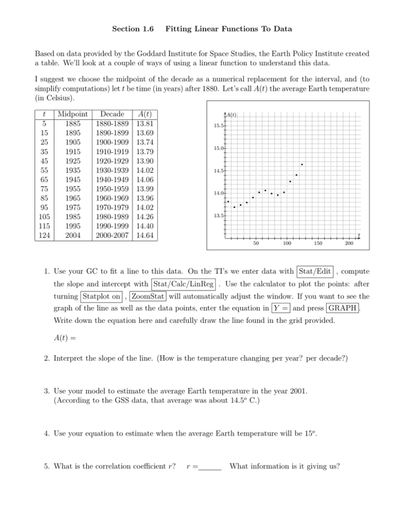
Section 1.6
Fitting Linear Functions To Data
Based on data provided by the Goddard Institute for Space Studies, the Earth Policy Institute created
a table. We’ll look at a couple of ways of using a linear function to understand this data.
I suggest we choose the midpoint of the decade as a numerical replacement for the interval, and (to
simplify computations) let t be time (in years) after 1880. Let’s call A(t) the average Earth temperature
(in Celsius).
.
.......
t
Midpoint
Decade
A(t)
5
1885
1880-1889 13.81
15
1895
1890-1899 13.69
25
1905
1900-1909 13.74
35
1915
1910-1919 13.79
45
1925
1920-1929 13.90
55
1935
1930-1939 14.02
65
1945
1940-1949 14.06
75
1955
1950-1959 13.99
85
1965
1960-1969 13.96
95
1975
1970-1979 14.02
105
1985
1980-1989 14.26
115
1995
1990-1999 14.40
124
2004
2000-2007 14.64
A(t)
15.5
15.0
•
14.5
•
•
•
14.0
•
•
•
•
•
•
•
•
•
13.5
t
..........
50
100
150
200
1. Use your GC to fit a line to this data. On the TI’s we enter data with Stat/Edit , compute
the slope and intercept with Stat/Calc/LinReg . Use the calculator to plot the points: after
turning Statplot on , ZoomStat will automatically adjust the window. If you want to see the
graph of the line as well as the data points, enter the equation in Y = and press GRAPH .
Write down the equation here and carefully draw the line found in the grid provided.
A(t) =
2. Interpret the slope of the line. (How is the temperature changing per year? per decade?)
3. Use your model to estimate the average Earth temperature in the year 2001.
(According to the GSS data, that average was about 14.5o C.)
4. Use your equation to estimate when the average Earth temperature will be 15o .
5. What is the correlation coefficient r?
r=
What information is it giving us?