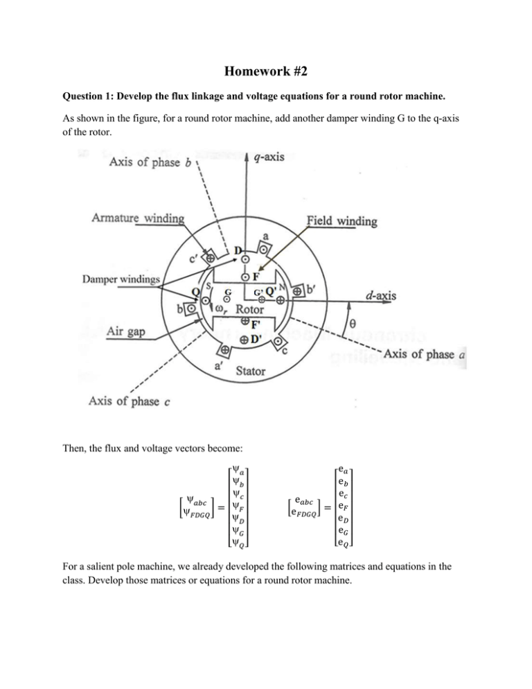
Homework #2
Question 1: Develop the flux linkage and voltage equations for a round rotor machine.
As shown in the figure, for a round rotor machine, add another damper winding G to the q-axis
of the rotor.
Then, the flux and voltage vectors become:
𝑎
𝑏
𝑐
𝑎𝑏𝑐

[
]= 𝐹
𝐹𝐷𝐺𝑄
𝐷
𝐺

[ 𝑄]
e𝑎
e𝑏
e𝑐
e𝑎𝑏𝑐
[e
] = e𝐹
𝐹𝐷𝐺𝑄
e𝐷
e𝐺
e
[ 𝑄]
For a salient pole machine, we already developed the following matrices and equations in the
class. Develop those matrices or equations for a round rotor machine.
Ls + Lm cos2

LSS = −Ms − Lmcos2 ( + )
6
5
[−Ms − Lmcos2 ( + 6 )
MFcos
LSR
= MFcos ( −
[MFcos ( +
d
Ld
q
0
0
0
− = −
F
𝑘MF
D
𝑘MD
[Q ] [ 0

−Ms − Lmcos2 ( + )
6
2
Ls + Lm cos2( − )
3

−Ms − Lmcos2 ( − )
2
MDcos
2
)
3
2
3
)
0
Lq
0
−
0
0
𝑘MQ
MDcos ( −
MDcos ( +
0
0
L0
−
0
0
0
|
|
|
|
|
|
|
𝑘MF
0
0
−
LF
MR
0
5
)
6

−Ms − Lmcos2 ( − )
2
2
Ls + Lm cos2( + ) ]
3
−Ms − Lmcos2 ( +
−MQsin
2
)
3
2
3
)
−MQsin ( −
−MQsin ( +
2
)
3 ,
2
3
𝑘MD
0
0
−
MR
LD
0
0
−id
𝑘MQ
−iq
0
−i0
−  −
iF
0
i
0
D
L Q ] [ iQ ]
LRR
)]
R a + 3R n
0
0
Ra
0
0
0
0
−𝑟 Lq
0
−𝑟 𝑘MQ
0
0
0
0
0
0
𝑟 Ld
0
RF
0
𝑟 𝑘MF
0
0
RD
𝑟 𝑘MD
0
0
0
Ra
0
0
0
0
RQ
𝑒0
𝑒𝑑
𝑒𝐹
𝑒𝐷 =
𝑒𝑞
𝑒
[ 𝑄]
[
0
LF M R 0
= [M R L D 0 ]
0
0 LQ
L0 + 3Ln
Ld
𝑘MF
𝑘MD
𝑘MF
LF
MR
𝑘MD
MR
LD
Lq
𝑘MQ
𝑘MQ
[
cos
cos ( −
2
LQ ]
2
For Park’s transformation, use P = √3 −sin −sin ( −
[ 1/√2
1/√2
)
3
2
3
)
]
−𝑖0
−𝑖𝑑
𝑖𝐹
𝑖𝐷 +
−𝑖𝑞
[ 𝑖𝑄 ]
−𝑖0
−𝑖𝑑
𝑖𝐹
d 𝑖 /dt
𝐷
−𝑖𝑞
[ 𝑖𝑄 ]
cos ( +
2
−sin ( +
1/√2
)
3
2
3
)
]
Question 2: Calculate id, iq and i0 under a disturbance
The rotor speed of a synchronous machine is measured for t=0~4 seconds as given in the table
below. The machine experiences a disturbance to cause a swing in the rotor’s speed, as shown by
the figure. Still, we assume three phase currents to be
ia= sinst
ib= sin(st - 2/3)
ic= sin(st + 2/3)
where s=260 rad/s. At t=0s, if the rotor position (0)=0rad, then calculate values of id, iq and
i0 at t=0.4s, 1.4s, 2.2s, 3.0s, and draw those values vs. time in one plot to show how the dq0
currents change under that disturbance.
t (s)
0
0.2
0.4
0.6
0.8
1
1.2
1.4
1.6
1.8
2
2.2
2.4
2.6
2.8
3
3.2
3.4
3.6
3.8
4
r (rad/s)
376.99112
376.99112
376.99112
376.99112
376.99112
376.99112
374.98090
374.81084
375.52963
376.38565
376.99112
377.26317
377.28619
377.18891
377.07306
376.99112
376.95430
376.95119
376.96435
376.98003
376.99112
377.5
377
Omegas
376.5
Omegar
376
375.5
375
374.5
0
0.5
1
1.5
2
Time (s)
2.5
3
3.5
4