masses, springs, washboarding cars.
Math 2280-2
March 6, 2001
Part I: two equal masses suspended with three identical springs:
> restart:with(linalg):
Warning, the protected names norm and trace have been redefined and unprotected
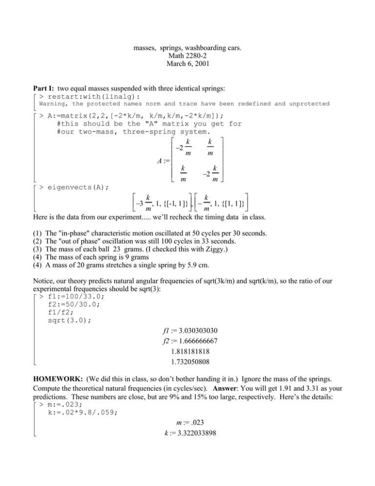
> A:=matrix(2,2,[-2*k/m, k/m,k/m,-2*k/m]);
#this should be the "A" matrix you get for
#our two-mass, three-spring system.

k
k 

 −2

m
m 


A := 

 k
k 

−2 
 m
m
> eigenvects(A);

  k
 k
 −3 , 1, {[-1, 1 ]},  − , 1, {[1, 1 ]}

  m
 m
Here is the data from our experiment..... we’ll recheck the timing data in class.
(1)
(2)
(3)
(4)
(4)
The "in-phase" characteristic motion oscillated at 50 cycles per 30 seconds.
The "out of phase" oscillation was still 100 cycles in 33 seconds.
The mass of each ball 23 grams. (I checked this with Ziggy.)
The mass of each spring is 9 grams
A mass of 20 grams stretches a single spring by 5.9 cm.
Notice, our theory predicts natural angular frequencies of sqrt(3k/m) and sqrt(k/m), so the ratio of our
experimental frequencies should be sqrt(3):
> f1:=100/33.0;
f2:=50/30.0;
f1/f2;
sqrt(3.0);
f1 := 3.030303030
f2 := 1.666666667
1.818181818
1.732050808
HOMEWORK: (We did this in class, so don’t bother handing it in.) Ignore the mass of the springs.
Compute the theoretical natural frequencies (in cycles/sec). Answer: You will get 1.91 and 3.31 as your
predictions. These numbers are close, but are 9% and 15% too large, respectively. Here’s the details:
> m:=.023;
k:=.02*9.8/.059;
m := .023
k := 3.322033898
> evalf(sqrt(k/m)/(2*Pi));
evalf(sqrt(3*k/m)/(2*Pi));
1.912750143
3.312980432
EXPLANATION: The springs actually have mass, equal to 9 grams each, which you did not take into
account. This is on the same order of magnitude as the ball masses, and causes the actual experiment to
run more slowly than our model predicts. In order to be more accurate the total energy of our model
must account for the kinetic energy of the springs. You actually have the tools to model this
more-complicated situation, using the ideas of total energy discussed in section 5.6, and a little Calculus.
I carried out such an analysis, assuming that the spring velocity at a point on the spring linearly
interpolates the velocity of the wall and mass (or mass and mass) which bounds it. Based on this
analysis, the improved model predicts the two fundamental frequencies to be 1.68 cycles per second and
2.99 cycles per second. This agrees with our experimental results to within 1%, which is pretty amazing.
I offer a prestigeous Math Department T-shirt to the first student or group of students to submit
this "corrected" model and results, including its derivation.
Part 2: Washboarding revisited. (The two-axle automobile page 332)
> restart:with(linalg):
Warning, the protected names norm and trace have been redefined and unprotected
Here is the matrix A which we deduce from equation 40 on page 332.
> A:=matrix(2,2,[-(k1+k2)/m, (k1*L1 - k2*L2)/m,
(k1*L1-k2*L2)/In, -(k1*L1^2+k2*L2^2)/In]);

k1 + k2
k1 L1 − k2 L2 

 −


m
m



A := 

2
2
 k1 L1 − k2 L2
k1
L1
+
k2
L2


−




In
In
Let’s do the system which results from the data in #24):
> m:=100;
In:=1000;
L1:=6;
L2:=4;
k1:=2000;
k2:=2000;
m := 100
In := 1000
L1 := 6
L2 := 4
k1 := 2000
k2 := 2000
> eigenvects(A);
  
 
4 1
4 1



 −72 + 4 74 , 1, { 1, − +
74  },  −72 − 4 74 , 1, { 1, − −
74  }
  
 
5 10
5 10



> evalf(%);
[-37.59069893, 1., {[1., .0602325267 ]}], [-106.4093011, 1., {[1., -1.660232527]}]
> pi:=evalf(Pi);
π := 3.141592654
> f1:=sqrt(37.59069893)/(2*pi);
f2:=sqrt(106.4093011)/(2*pi);
f1 := .9757989175
f2 := 1.641760970
> fforce:=v/L;
#forcing requency is speed divided
#by wavelength of washboard (more like freeway
#syndrome than off-road case here...
v
fforce :=
L
> L:=40;
solve(f1=v/L,v);
solve(f2=v/L,v);
#critical car speeds in feet/sec
L := 40
39.03195670
65.67043880
> 39.03195670*(1/5280)*3600;
65.67043880*(1/5280)*3600;
#speeds in miles/hour
26.61269775
44.77529920