election2006.nb
1
This is a classroom example related to the 2006 elections and should be viewed as a simple comparison of the relative poll
standings of the top two candidates, versus how they fared in the vote, in 19 different gubanatorial races and 17 different
national senatorial races.
For each race, data was available from a poll close to the election and the sample size of the poll was known. In all but one
of these races the leader in the poll won the election. One gubanatorial poll was reported as a tie.
A number of the gubanatorial polls had sample size 500. Many of those bore the name of a small private polling organization
and were conducted less close to the election.
11 of the 19 gubanatorial polls underestimated the final vote of the eventual winner.
8 of the 17 senatorial polls underestimated the final vote of the eventual winner.
The data format is {a, b, c, d, e} with
a = % of poll vote for the election winning candidate
b = % of poll vote for the candidate placing second
c = % of election vote for the election winning candidate
d = % of election vote for the candidate placing second
e = sample size n of the poll
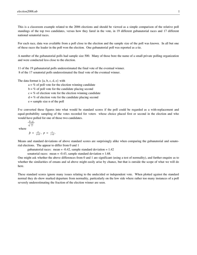
I've converted these figures into what would be standard scores if the poll could be regarded as a with-replacement and
equal-probability sampling of the votes recorded for voters whose choice placed first or second in the election and who
would have polled for one of those two candidates.
p` - p
ÅÅÅÅÅÅÅÅ
ÅÅÅÅÅÅÅ
pq
"########
ÅÅÅÅnÅÅ ÅÅ
where
a
c
p` = ÅÅÅÅ
ÅÅÅÅÅÅ , p = ÅÅÅÅ
ÅÅÅÅÅ .
a+b
c+d
Means and standard deviations of above standard scores are surprisingly alike when comparing the gubanatorial and senatorial elections. The appear to differ from 0 and 1
gubanatorial races: mean = -0.42, sample standard deviation = 1.42
senatorial races: mean = -0.43, sample standard deviation = 1.68.
One might ask whether the above differences from 0 and 1 are significant (using a test of normality), and further enquire as to
whether the similarities of emans and sd above might easily arise by chance, but that is outside the scope of what we will do
here.
These standard scores ignore many issues relating to the undecided or independent vote. When plotted against the standard
normal they do show marked departure from normality, particularly on the low side where rather too many instances of a poll
severely underestimating the fraction of the election winner are seen.
election2006.nb
2
42
i
j
j
j
j
51
j
j
j
j
j
53
j
j
j
j
j
51
j
j
j
j
j
50
j
j
j
j
j
52
j
j
j
j
j
j
50
j
j
j
j
j
53
j
j
j
j
j
52
j
j
j
j
51
gov2 = j
j
j
j
j
j
j
61
j
j
j
j
j
45
j
j
j
j
j
61
j
j
j
j
j
51
j
j
j
j
j
69
j
j
j
j
j
j
55
j
j
j
j
j
55
j
j
j
j
j
58
j
j
j
k 48
i 48
j
j
j
j
45
j
j
j
j
j
48
j
j
j
j
j
47
j
j
j
j
j
38
j
j
j
j
j
41
j
j
j
j
j
j
44
j
j
j
j
j
44
j
j
j
j
sen2 = j
49
j
j
j
j
j
40
j
j
j
j
j
39
j
j
j
j
j
j 38
j
j
j
j
j
41
j
j
j
j
j
35
j
j
j
j
j
47
j
j
j
j
j
j 44
j
j
k 31
40
42
38
39
42
43
47
29
42
43
26
45
33
38
24
38
38
35
45
51
53
49
50
58
59
54
56
50
50
58
60
57
60
53
53
67
48.52
55.77
55.77
56.33
52.18
53.99
53.21
55.56
56.35
47.92
68.69
46.69
62.75
57.8
69.01
60.36
60.36
60.26
52.77
47
41
44
46
34
44
46
42
44
38
43
35
44
31
45
41
31
48
50
49
49
54
48
49
54
52
50
52
58
50
60
48
49
64
40.73
40.76
39.14
40.87
45.11
45.11
45.63
35.22
42.32
43.92
31.31
45.73
35.24
38.35
29.15
29.15
36.84
39.74
45.33
677
520
602
594
747
800
663
436
741
676
800
1200
1200
553
880
625
1502
y
z
z
z
z
z
z
z
z
z
z
z
z
z
z
z
z
z
z
z
z
z
z
z
z
z
z
z
z
z
z
z
z
z
z
z
z
z
z
z
z
;
z
z
z
z
z
z
z
z
z
z
z
z
z
z
z
z
z
z
z
z
z
z
z
z
z
z
z
z
z
z
z
z
z
z
z
z
z
z
z
{
747
549
500
500
500
756
663
500
1200
500
500
710
625
800
500
500
646
646
800
y
z
z
z
z
z
z
z
z
z
z
z
z
z
z
z
z
z
z
z
z
z
z
z
z
z
z
z
z
z
z
z
z
z
z
z
z
z
z
z
z
z
z
z
z
z
;
z
z
z
z
z
z
z
z
z
z
z
z
z
z
z
z
z
z
z
z
z
z
z
z
z
z
z
z
z
z
z
z
z
z
z
z
z
z
z
z
z
z
z
z
z
{
Length@gov2D
19
Length@sen2D
17
compare@x_D := Module@8phat = x@@1DD ê Hx@@1DD + x@@2DDL, p = x@@3DD ê Hx@@3DD + x@@4DDL<,
Hphat - pL ê Sqrt@p H1 - pL ê x@@5DDDD
phi@r_, sig_D := Exp@-r ^ 2 ê H2 sig ^ 2LD ê Hsig Sqrt@2 PiDL
election2006.nb
3
gov2z = Table@compare@gov2@@iDDD, 8i, 1, 19<D 1.0
8-1.72552, -1.39283, -0.23583, -0.582536, 0.320318,
0.141632, -1.18179, 1.57453, -1.25316, 0.930022, 0.687059, -0.276795,
0.446179, -1.62373, 1.90366, -3.95756, -1.55021, 1.09361, -1.23627<
11 of 19 gubanatorial polls underpredicted the vote for the candidate leading in the poll (negative gov2z scores).
8Mean@gov2zD, Sqrt@H19 ê 18L HMean@gov2z ^ 2 - Mean@gov2zD ^ 2DLD<
8-0.416802, 1.41899<
sen2z = Table@compare@sen2@@iDDD, 8i, 1, 17<D 1.0
8-0.514603, 0.395721, 1.06772, 0.0158769, 0.531548, -3.86507, -1.81521, 0.105228, 2.00044,
0.662757, -2.87358, 0.815924, -3.45159, 1.37751, -0.823387, -0.0977524, -0.825698<
8 of 17 senatorial polls underpredicted the vote for the candidate leading in the poll (negative sen2z scores).
8Mean@sen2zD, Sqrt@H19 ê 18L HMean@sen2z ^ 2 - Mean@sen2zD ^ 2DLD<
8-0.429069, 1.68089<
Here is a plot of the gubanatorial standard scores shown together with the standard normal.
Show@Plot@Mean@phi@r - gov2z, 0.4DD, 8r, -5, 5<D, Plot@phi@r, 1D, 8r, -4, 4<DD
0.3
0.25
0.2
0.15
0.1
0.05
-4
-2
2
4
0.4
0.3
0.2
0.1
-4
-2
2
4
election2006.nb
4
0.4
0.3
0.2
0.1
-4
-2
2
4
Ü Graphics Ü
Here is a plot of the senatorial standard scores shown together with the standard normal.
Show@Plot@Mean@phi@r - sen2z, 0.4DD, 8r, -5, 5<D, Plot@phi@r, 1D, 8r, -4, 4<DD
0.3
0.25
0.2
0.15
0.1
0.05
-4
-2
2
4
0.4
0.3
0.2
0.1
-4
-2
2
4
election2006.nb
5
0.4
0.3
0.2
0.1
-4
Ü Graphics Ü
-2
2
4