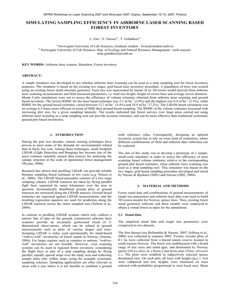
ISPRS Workshop on Laser Scanning 2007 and SilviLaser 2007, Espoo, September 12-14, 2007, Finland
SIMULATING SAMPLING EFFICIENCY IN AIRBORNE LASER SCANNING BASED
FOREST INVENTORY
L. Ene a, E. Næsset b , T. Gobakken b
a
b
Norwegian University of Life Sciences, Graduate student - liviue@student.umb.no
Norwegian University of Life Sciences, Dep. of Ecology and Natural Resource Management - (erik.naesset,
terje.gobakken)@umb.no
KEY WORDS: Airborne laser scanner, Simulator, Forest inventory
ABSTRACT:
A simple simulator was developed to test whether airborne laser scanning can be used as a strip sampling tool for forest inventory
purposes. The simulator is based on the existing two stages, grid based laser inventory procedure. A population of trees was created
using an existing forest stand structure generator. Each tree was represented by means of its 3D-crown model derived from airborne
laser scanning measurements and field measured parameters, i.e. total tree height, height of crown base and average crown diameter.
Monte Carlo simulations were run to assess the efficiency of volume estimates obtained from airborne laser scanning and ground
based inventory. The lowest RMSE for the laser based estimates was 5.1 m3ha-1 (2.0%) and the highest was 8.4 m3ha-1 (3.3%), while
RMSE for the ground based estimates varied between 13.7 m3ha-1 (5.4%) and 18.4 m3ha-1 (7.2%). The LIDAR based estimation was
on average 6.3 times more efficient in terms of MSE than ground based sampling. The RMSE of the volume estimates increased with
increasing plot size, for a given sampling intensity. The results indicated that forest surveys over large areas carried out using
airborne laser scanning as a strip sampling tool can provide accurate estimates, and can be more effective than traditional systematic
ground plot based inventories.
truth reference value. Consequently, designing an optimal
inventory system has to rely on some kind of simulation, where
different combinations of field and airborne data collection can
be explored.
1. INTRODUCTION
During the past two decades, remote sensing techniques have
proven to meet some of the demand for environmental related
data at fairly low cost. Among these techniques, small footprint
LIDAR (LIght Detection and Ranging) has become one of the
most common remotely sensed data sources for analyzing the
canopy structure at the scale of operational forest management
(Wynne, 2006).
The aim of this study was to develop a prototype of a simple,
small-scale simulator in order to assess the efficiency of laser
scanning based volume estimates relative to the corresponding
ground plot based estimates, when airborne laser scanning was
used as a strip sampling tool. This simulator was based on the
two stages, grid based sampling procedure developed and tested
by Næsset & Bjerknes (2001) and Næsset (2002, 2004).
Research has shown that profiling LIDAR can provide reliable
biomass sampling based estimates at low costs (e.g. Nelson et
al., 2006). The LIDAR based procedure consists of a two stage
sampling scheme. LIDAR transects are taken by flying parallel
fight lines separated by many kilometers over the area in
question. Systematically distributed ground plots or ground
transects are measured along the LIDAR transect. Ground based
estimates are regressed against LIDAR measurements, and the
resulting regression equation are used for prediction along the
LIDAR transects across the entire sampled area (Nelson et al.,
2004).
2. MATERIAL AND METHODS
Forest stand data and combinations of ground measurements of
single tree parameters and airborne laser data were used to build
3D crown models for Norway spruce trees. Then, existing forest
stand generator software and these models were employed to
obtain a virtual forest as input for the simulations.
In contrast to profiling LIDAR systems which only collects a
narrow line of data on the ground, commercial airborne laser
scanners provide an accurately geolocated cloud of 3dimensional observations, which can be related to ground
measurements such as plots of various shapes and sizes.
Scanning LIDAR is today used operationally for stand-based
“wall-to-wall” inventories of forest stands in Norway (Næsset,
2004). For larger regions such as counties or nations, “wall-towall” inventories are not feasible. However, even scanning
systems can be used in regional forest inventory, considering
the flight lines as part of a strip sampling design by flying
parallel, equally spaced strips over the study area and collecting
sample plots only within strips, using for example systematic
sampling schemes. Sampling applications are often relevant in
areas with a size where it is not feasible to establish a ground
2.1 Stand data
The empirical stand data and single tree parameters were
comprised in two datasets.
The first dataset (see Bollandsås & Næsset, 2007; Solberg et al.,
2006) was collected in summer 2003. Twenty circular plots of
0.1 ha were collected from a boreal nature reserve located in
south-eastern Norway. The forest was multilayered with a broad
range of tree sizes and stand ages, and dominated by Norway
spruce [Picea abies (L.) Karst.] and Scots pine (Pinus silvestris
L.). The plots were establish in subjectively selected spruce
dominated sites. On each plot, all trees with height (dbh) ≥ 3cm
were callipered and tree heights were measured on trees
selected with probability proportional to stem basal area. Mean
114
IAPRS Volume XXXVI, Part 3 / W52, 2007
diameter was defined as diameter corresponding to mean stem
basal area (dBA) and mean height was defined as the average
basal area weighted (Lorey’s) height (hL).
the mean of planimetric coordinates, and then the resulted laser
point clouds were considered as spatial crown models for
Norway spruce trees. Laser pulses with heights below 2 m were
considered as ground points.
Both Global Positioning System (GPS) and Global Navigation
Satellite System (GLONASS) were used to determine the
planimetric coordinates (Euref89) of the plot centers. The
average estimated accuracy of the plot coordinates was 10 cm.
The relationships between field and laser measurements were
established for a total of 435 spruce trees. Hence, each of these
trees were represented as unique combinations of diameter (dbh),
height (h), crown height (ch), crown projection radius (cr), stem
volume (v) (Table 1), and the associated 3D crown models. For
each of these trees, the volume was calculated by the means of
functions for Norway spruce with bark (Vestjordet 1967).
Further in this study, the trees were called “single tree models”.
For the first dataset, polar coordinates from the plot centre were
registered for all trees with dbh ≥ 3 cm. Total tree height, height
of crown base, crown radius in four cardinal directions, and
average crown diameter were measured on trees selected from
each plot. The final coordinates for all single trees were
computed in Euref89, using plot centre coordinates and plotwise polar tree coordinates.
The second dataset (see Næsset, 2004) comprised 60 large plots
located in a productive forest area of approximately 5000 ha in
the municipality of Krødsherad, south-eastern Norway. The
forest composition was dominated by Norway spruce and Scots
pine, while younger stands were dominated by deciduous
species, mainly birch (Betula pubescens Ehrh.). The plot areas
were from 3121 to 4219 m2, with an average of 3739 m2. Within
each plot, all trees with diameter at breast height dbh ≥ 4 cm and
dbh ≥ 10 cm were callipered in young and mature stands,
respectively, using 2 cm diameter classes. Height measurements
were taken from trees selected with probability proportional to
stem basal area at breast height. For each plot, the mean height
corresponding to Lorey’s height was computed from the mean
height of the individual diameter classes, weighted by total plot
basal area for each diameter class.
Metrics Mean S.D.
Min
dbh (cm)
3.2
19.8
10.4
Median Max
18.8
51
h (m)
15.8 6.1
3.6
16
29.5
ch(m)
3.4
2.4
0.2
3.1
13.5
cr (m)
1.3
0.4
0.6
1.3
2.9
v (m3) 0.38 0.41 0.003 0.22 2.46
a
dbh-diameter; h-height; ch–crown height; cr–crown radius;
v-volume; S.D.-standard error
Table 1. Descriptive statistics for individual tree model
parameters a.
2.4 Virtual forest
The program package SILVA 2.2 (Pretzsch et al., 2002) was
used to generate a virtual forest. The stand generator provides a
tree list with associated parameters. For each tree, the following
information was recorded: tree species, diameter at breast
height, total height and height of crown base, crown diameter
and tree coordinates (x, y). To generate the tree lists, the input
parameters were tree species, dBA (cm), dmax (cm), hL (m), and
N, obtained from ground measurements. Only 13 plots from the
first dataset and 25 plots from the second dataset provided
acceptable combinations of input parameters which could be
used to obtain tree lists by means of SILVA 2.2 (Tab. 2). The
other plots were rejected due to inadvertencies between the test
plot reference data and model calibration of the stand generator.
Totally, a number of 38 tree lists were obtained and each of
them was considered as a possible realization of a forest stand,
given the ground-measured input parameters.
2.2 Laser data
Laser scanner data were acquired during June 2005 (leaf-on
canopy condition) from the same area as the first dataset, with
an Optech ALTM 3100 sensor operating at 100 kHz laser pulse
repetition rate and 70 Hz scanning frequency. The aircraft was
flown approximately 750 m above ground with an average
speed of 75 ms-1. The maximum half scan angle was 10°, and
the corresponding swath width was about 264 m. Pulses
transmitted at scan angles that exceeded 8° were excluded from
the final dataset. The average footprint size was about of 21 cm,
with an average point density of 5.09 m-2. First and last echo
were recorded.
2.3 Laser-derived single tree models
The virtual forest study area was defined in a 2D-local
coordinate system with axes being multiples of 100 m, and the
terrain was assumed to be flat. The frame of study area was
considered to be a two-dimensional array, where each (i, j)
position is a squared area representing a forest stand of 1.0 ha.
Laser data and the ground measurements collected in summer
2003 from 0.1 ha stand plots comprised into the first dataset
were used to obtain crown representation of Norway spruce
trees. Laser pulse hits were related to tree crown projections by
Stand parameters
First dataset (0.1 ha plots)
Second dataset (large plots)
dBA s dmax s hL s
Ns
dBA s dmax s hL s
Ns dBA p dmax p hL p Np dBA b dmax b
Max
30.1
60.6 28.9 1040 27.6
51
22.2 904 36.3
49
23.6 622 23.9
47
Min
19.9
39.6 17.7 650
12
17
8.4
13
18.7
35
12.7 10
11.5
13
Mean 17.2
37.3
17
671
17.4
32.1 14.9 360 21.6
35.5
14.4 229 12.6
21.7
a
dBA=basal area mean diameter (cm); dmax=maximum diameter (cm); hL=basal area weighted mean height (m);
N=stem number per ha; s=Norway spruce; p=Scots pine; b =deciduous trees (assimilated with birch).
hL b
20
10.8
10.6
Table 2. Summary of stand metrics for 13 selected plots from the first dataset and 25 plots from the second dataset a.
115
Nb
286
5
82
ISPRS Workshop on Laser Scanning 2007 and SilviLaser 2007, Espoo, September 12-14, 2007, Finland
based systematic plot sampling estimates was assessed for each
sampling scheme.
To create the population, one of the 38 virtual forest stands of
1.0 ha generated by means of SILVA 2.2 was randomly
allocated to each (i, j) array position, and then the stand
coordinates for each tree were translated according to the new
location within the array. The neighborhood effects among
forest stands were ignored. Thus, the spatial structure of each
cell was supposed to be independent of the position in the array.
The study area was defined as a square of 36 km2.
Computations
Multiple regression analysis was used to establish stratumspecific relationships between field measurements and laser
derived metrics. Based on previous findings (e.g. Magnussen &
Boudewyn, 1998; Næsset, 1997, 2002, 2004), two independent
variables derived form first laser pulse returns were used for
volume prediction within each grid cell: the percentile
corresponding to the 9th quantile of laser canopy height (h90)
considering the lowest canopy height (≥2m), and the canopy
density corresponding to the proportion of the first pulse laser
hits (d0). Canopy density was defined as the proportions of first
pulse laser hits above 2 m to total number of first pulse returns.
To calculate the canopy density, it was necessary to find the
total number of laser hits within each grid cell. Because the last
echoes from initial laser scanning data were not available, it was
assumed that each grid cell had a uniform coverage of laser hits.
Thus, the total number of laser hits within a grid cell could be
linearly extrapolated from the number of hits that fall inside the
crown projection. Laser hits with heights below 2 m were
considered as ground points as well.
Further, each tree from the tree list was substituted with a
diameter-equivalent single tree model. Because of the relatively
small number of single tree models (i.e. 435 trees) which could
be derived from available dataset, only dbh was used as key. The
rest of the single tree model parameters, i.e. height, crown
height, crown radius, laser pulse heights, and stem volumes,
were then transferred to the corresponding diameter-equivalent
trees from the tree list positioned at (xi, yi) coordinates in the
study area. The matching results often consisted of more than
one single tree model with equal diameters. In this situation,
only one of these tree models was randomly selected to replace
the tree at the position (xi, yi) from the generated forest stand.
For the situations when diameter matching did not occur- which
means that some trees from generated forest stands have
diameters that were not among the diameters of single tree
models, a single tree model with diameter closest to the missing
value, either larger or smaller, was selected instead. Thus, the
study area was re-populated with laser derived tree models, and
the volume of the entire population was calculated as the sum of
individual trees.
The full second order regression model based on these variables
was subject to stepwise variable selection to develop final
models for prediction. Exploratory regression analysis was run
to detect possible deviations from model assumptions. Various
variance stabilizing transformations of the dependent variable
(sample plot volume) were analytically assessed by the means
of the Box-Cox method. Five regression models were finally
proposed: (1) a multiplicative model, (2) a linear model without
transformations, and three different models with transformed
response variable: (3) log(y), (4) sqrt(y), and (5) asin(sqrt(y)).
For the multiplicative model, only two independent variables
(h90 and d0) were used, and consequently this model was not
subject to stepwise selection.
For other species than Norway spruce, i.e. Scots pine and birch,
there were no available laser data for building 3D crown
models. For this reason, diameter matching was done regardless
of species, which means that trees of different species could be
matched if they had the same diameter. After diameter
matching, trees from the tree list generated by means of forest
stand generator were replaced with diameter equivalent Norway
spruce single tree models, regardless tree species.
For the other regression models, an empirical approach was
used to obtain regression equations. Before each simulation, a
number of 20 iterations were used to select the final regression
models. First, a stripe sampling scheme was randomly generated
over the study area, and the location of each stripe and
correspondent sample plots were hold fixed. Initial sampling
trials were run, and for each iteration a new population outcome
was generated and sampled. Stepwise regression (pin = 0.05, pout
= 0.10) was used for model selection, and each resulted subset
model was registered. After running all iterations, the most
frequently used model form for each regression model was
selected as final model to be used for prediction during
sampling simulations. Since serious muliticollinearity problems
occurred, best subsets regression models were also derived and
compared to the stepwise regression subsets, in order to select
unbiased regression models.
Laser scanning data consist of clouds of laser hits related to tree
crowns. In this study, each laser hit (first echo) has known x, y
and z-coordinates, but in this analysis, the (xi, yi) coordinates of
each laser hit were discarded. It was assumed that laser hits
related to trees inside a grid cell fall inside the same cell where
these trees are located, and that all the hits inside a tree crown
projection belong only to that tree.
2.5 Simulator
The strip sampling simulation was based on the two-stage
procedure described by Næsset & Bjerknes (2001) and Næsset
(2002, 2004) and follows the approach proposed by Gobakken
et al. (2006). In parallel, an estimation of mean volume by
means of ground plot systematic sampling was done, as a kind
of conventional inventory. The sampling units consist of equal
strips containing the same number of grid cells. The total
volume was estimated as the sum of predicted volume for all
grid cells over all strips. Monte Carlo (MC) estimates of
population mean volume and sampling error were derived
running 50 iterations for each sampling scheme. Bias, standard
deviation and RMSE for estimated mean values were used to
assess the sampling estimates against the reference volume of
the predefined population. The systematic samples of laser
scanning strips and ground plots were treated as random
samples. Relative efficiency of regression based estimates
obtained from laser scanning strip sampling against ground
To estimate the population volume, Monte Carlo experiments
were run to derive laser scanning and ground-based mean
volume estimates. Initial tests showed that cumulated mean
volume estimates over 50 iterations converged towards the
value of MC estimates, while the sampling error decreased
asymptotically. However, the number of iterations should vary
with the study area, sample design, and population variability.
Squared sample plots of 200, 400, and 600 m2 were used to
provide ground estimates. Using squared plots significantly
improves the computational performance during simulation.
116
IAPRS Volume XXXVI, Part 3 / W52, 2007
Parallel laser strips with widths of 160, 180, and 200 m spaced
at 1500 m were generated. The sampling intensity for different
plot sizes was held almost constant around 0.6% of stripe
sampling area, and the sample size varied with plots size.
Compared to sampling intensities in ongoing research studies,
which typically are less than 0.003% (Gobakken et al., 2006),
the sampling intensity at stand plots level is much higher, but
necessary to reach ground samples large enough to get reliable
regression estimates.
16
Sampling error(m 3ha-1)
14
Finally, the MC estimates for both laser strip and ground based
systematic sampling were assessed by the means of a two-tailed
t-test against the population value. Bias, standard deviation, and
RMSE for the MC estimates of mean volume were then used to
assess the sampling designs and regression models. Relative
efficiency of regression based laser scanning estimates against
corresponding ground based estimates was calculated as ratio of
their respective MSE.
12
10
sampling error for laser-based estimates
sampling error for ground plot-based estimates
standard deviation for laser-based estimates
standard deviation for ground plot-based estimates
8
6
4
2
0
1
5
10
15
20
25
30
Iterations
35
40
45
50
Figure 3. Example of sampling error estimation, for
multiplicative regression model and ground plot base estimates
using strip width of 180 m and plot size of 400 m2.
4. RESULTS
Except the multiplicative model, final regression equations were
built using stepwise regression. A number of 45 mean volume
estimates and their RMSE values were derived using five
regression models (Table 4). In addition, for each sampling
scheme, an estimate of mean volume and the corresponding
RMSE were derived by ground based systematic plot sampling
(Table 4). The reference value of mean volume per ha was 254
m3, i.e., total population volume of 914,400 m3 divided by the
size of the study area of 3600 ha. The simulated study area
included over 2.7 million trees. The number of iterations used
for each simulation ensured convergence for both regression
and ground plot based estimates. For mean timber volume
estimates, the convergence occurred after ca 40-45 iteration for
sampling schemes using ground plots of 200 m2, ca 20-30
iterations for plots of 400 m2, and after ca 15-25 iterations for
plots of 600 m2. As the number of iterations increased, the
sampling error decreased asymptotically (Figure 1).
5. DISCUSSION
The major findings of this study indicated that:
1) Laser scanning-based stripe sampling forest inventory can
provide accurate and precise estimates of mean volume for
relatively large forest areas. The LIDAR based estimation was
on average 6.3 times more efficient in terms of MSE than
ground-based sampling.
2) For both inventory methods, the inverse relationship between
plot size and sample size seemed to be the dominant factors that
led to a general increase of RMSE as the plot size increased.
3) For the ground-based systematic plot sampling method, the
plot size was the dominant factor which led the overall trends
for the MC estimates of mean volume. The RMSE of volume
estimates increased by increasing plot size.
The regression models comprised two to five predictor
variables. The most frequently used prediction variable was the
interaction term, followed by squared height percentile and
canopy density. Generally, the R2 ranged between 0.79 and
0.96. The bias of mean volume estimates during iterations in
each simulation ranged between -16.6 m3ha-1 (6.5%) and 10.2
m3ha-1 (4.0%) for regression estimates, while the bias of ground
based estimates ranged from -34.1 m3ha-1 (13.4%) to
31.8 m3ha-1 (12.5%). MC estimates of mean volume derived by
regression ranged between -5.7 m3ha-1 (2.2%) and 0.3 m3ha-1
(0.1%), and standard error between 5.0 m3ha-1 (2.0%) and 7.4
m3ha-1 (2.9%). For plot-based MC estimates, the range of bias
was between -2.6 m3ha-1 (1.0%) and 3.9 m3ha-1 (1.5%), with a
standard error between 13.7 m3ha-1 (5.4%) and 18.4 m3ha-1
(7.2%). The lowest RMSE for regression based MC estimates
was 5.1 m3ha-1 (2.0%) and the highest was 8.4 m3ha-1 (3.3%).
RMSE for ground plot MC estimates varied from 13.7 m3ha-1
(5.4%) to 18.4 m3ha-1 (7.2%). Among all regression models,
only the multiplicative and linear models gave unbiased
estimates (p > 0.05) under all sampling schemes. Ground based
systematic plot sampling derived estimates provided unbiased
estimates (p >0.05) for all sampling designs. Relative efficiency
of laser based estimates relative to ground plot estimates varied
between 0.11 and 0.28, with an average of 0.16, which indicates
efficiency in average 6.3 times higher for laser scanning strip
sampling method (Table 5).
However, generalizations cannot be drawn from this study,
since many assumptions were not realistic compared to realworld applications, i.e. small size of target area and small
population variability. Another important issue is that all
metrics derived from the population were considered to be
“error free” and the effects of error propagation were neglected.
As possible error sources could be mentioned errors concerning
ground location of trees and ground plots, laser sampling and
field measurements.
Nevertheless, we believe development and application of this
first small-scale simulator has provided useful insight into some
of the challenges we will have to face in the continued work to
develop simulators that can operate on larger model forests
where also spatial correlation and regional trends in the
population value may be accounted for. Furthermore, a forest
stand generator calibrated for Norwegian conditions should be
developed, and there is also a need for building up an empirical
database of laser derived individual tree models for all main tree
species in Scandinavia.
117
ISPRS Workshop on Laser Scanning 2007 and SilviLaser 2007, Espoo, September 12-14, 2007, Finland
Strip
Plot area
width Model
(m)
1
160
180
200
160
2
2
200 m
400 m
600 m
bias S.D RMSE bias S.D RMSE bias S.D RMSE
Laser scanning based estimates (m3ha-1)
-0.8ns
5.5
5.6
-0.8ns
ns
5.7
(MSEa / MSEb)
Strip
2
5.8
-0.2ns
6.4
6.4
ns
width Model
(m)
Plot size (m2)
200
400
600
1
2
0.17 0.14 0.12
0.23 0.18 0.16
3
4
0.16 0.15 0.12
0.32 0.21 0.21
5
0.16 0.14 0.12
1
2
0.14 0.13 0.10
0.21 0.16 0.16
2
-2.2*
6.2
6.6
-1.3
6.4
6.5
-0.8
7.4
7.4
3
4
-1.5*
-5.5*
5.2
5.6
5.4
7.8
-1.6ns
-3.6*
5.7
6.1
5.9
7.1
-0.9ns
-4.3*
6.5
7.2
6.5
8.4
5
-0.6ns
5.5
5.5
-1.0ns
5.7
5.8
-0.5ns
6.3
6.4
1
-0.7ns
5.5
5.6
-0.7ns
5.0
5.1
-0.5ns
5.6
5.7
2
-3.0*
6.2
6.9
-0.4ns
5.7
5.8
-0.8ns
7.1
7.1
3
0.13 0.14 0.12
3
4
ns
-1.4
-5.7*
5.3
5.6
5.4
8.0
ns
-1.3
-3.6*
5.1
5.7
5.3
6.7
ns
-1.4
-4.1*
6.0
7.0
6.2
8.1
4
0.28 0.22 0.21
-0.5ns
5.4
5.0
5.1
-0.9ns
0.13 0.13 0.10
5.4
-0.8ns
5
5
5.5
5.6
1
-0.2ns
5.4
5.4
-0.1ns
5.1
5.1
-0.2ns
6.0
6.0
-2.5*
5.7
6.2
5.9
5.9
-0.7ns
0.13 0.12 0.11
0.18 0.16 0.15
2
0.3 s
1
2
7.2
7.2
3
4
ns
-0.9
-5.2*
5.1
6.4
ns
-1.2
-3.1*
6.3
7.1
6.4
7.7
3
4
0.13 0.12 0.12
0.27 0.19 0.18
0.0ns
5.4
5.4
-0.2ns 5.2
5.2
-1.0ns
Ground plot based inventory (m3ha-1)
5
0.13 0.13 0.11
5
6.0
6.1
-
5.3
5.7
-0.7ns 13.7
ns
5.4
7.7
13.7
ns
-0.7
-3.2*
5.0
5.5
3.9ns 14.9
ns
15.4
180
200
a
MSE of laser-based estimates
MSE of laser-based estimates
Models: 1–multiplicative; 2–log(y);
3– sqrt(y); 4–asin (sqrt(y)); 5-linear.
b
1.8ns 18.4
ns
160
18.4
180
-
-2.1
14.8
15.0
2.2
14.1
14.3
2.2
17.5
17.6
200
-
-2.6ns 14.5
14.8
2.2ns 14.5
14.7
2.2ns 18.2
18.4
a
significance level: * p < 0.05; not significant: ns > 0.05;
Models: 1–multiplicative; 2–log(y); 3–sqrt(y); 4–asin (sqrt(y)); 5-linear.
Table 5. Relative efficiency of laser
based against ground plot estimates.
Table 4. Bias, standard error (S.D) and RMSE of mean volume estimates (m3ha-1).
Næsset, E. and Bjerknes, K. 2001. Estimating tree heights and
number of stems in young forest stands using airborne laser
scanner data. Remote Sens. Environ., 78: 328-340.
REFERENCES
Bollandsås, O. M. and Næsset, E. 2007. Estimating percentilebased diameter distributions in uneven-sized Norway spruce
stands using airborne laser scanner data. Scand. J. For. Res.,
22:33-47.
Næsset, E., 2002. Predicting forest stand characteristics with
airborne scanning laser using a practical two-stage procedure
and field data. Remote Sens. Environ., 80: 88-99.
Gobakken, T., Næsset, E. and Nelson, R. 2006. Developing
regional inventory procedures based on scanning LiDAR. In:
Hirata, Y., Awaya, Y., Takahashi, T., Sweda, T. & Tsuzuki, H.
(Eds.). Proceedings of the Silvilaser 2006 Conference,
Matsuyama, Japan. Pp 99-104.
Næsset, E. 2004. Practical large-scale forest stand inventory
using small-footprint airborne scanning laser. Scand. J. For.
Res., 19: 164-179.
Pretzsch, H., Biber, P. and Ďursky, J. 2002. The single treebased stand simulator SILVA: construction, application and
evaluation. For. Ecol. Manage., 162: 3-21.
Magnussen, S. and Boudewyn, P. 1998. Derivations of stand
heights from airborne laser scanner data with canopy-based
quantile estimators. Can. J. For. Res., 28: 1016-1031.
Solberg, S., Næsset, E. and Bollandsås, O.M. 2006. Single tree
segmentation using airborne laser scanner data in a structurally
heterogeneous spruce forest. Photogramm. Eng. Remote
Sensing, 72: 1369-1378.
Nelson, R., Short, A. and Valenti, M. 2004. Measuring biomass
and carbon in Delaware using an airborne profiling LIDAR.
Scand. J. For. Res., 19: 500-511.
Nelson, R., Næsset, E., Gobakken, T., Ståhl, G. and Gregoire,
T.G. 2006. Regional forest inventory using airborne profiling
LiDAR. In: Hirata, Y., Awaya, Y., Takahashi, T., Sweda, T. &
Tsuzuki, H. (Eds.). Proceedings of the Silvilaser 2006
Conference, Matsuyama, Japan. Pp 105-112.
Vestjordet, E. 1967. Functions and tables for volume of
standing trees. Norway spruce. Rep. Norw. For. Res. Inst. 22:
539-574. (In Norwegian with English summary).
Wynne, R. H. 2006. Lidar remote sensing of forest resources at
the scale of management. Photogramm. Eng. Remote Sensing,
72:1311-1314.
Næsset, E. 1997. Determination of mean tree height of forest
stands using airborne laser scanner data. Photogramm. Eng.
Remote Sensing, 52: 49-56.
118