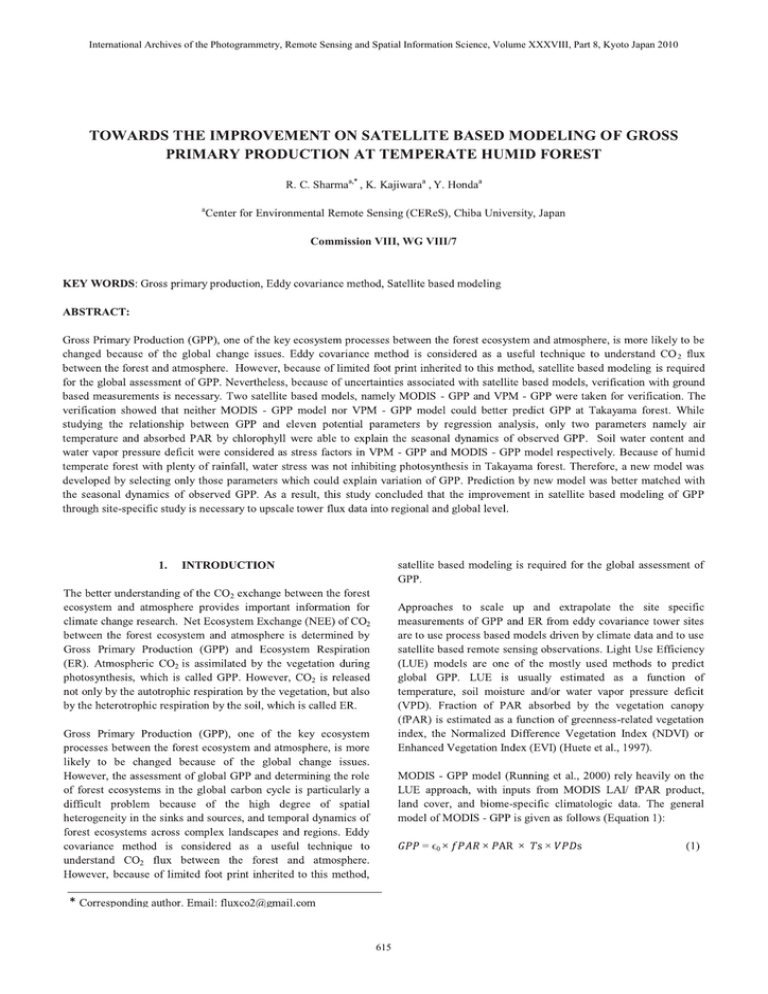
International Archives of the Photogrammetry, Remote Sensing and Spatial Information Science, Volume XXXVIII, Part 8, Kyoto Japan 2010
Commission VIII, WG VIII/7
615
International Archives of the Photogrammetry, Remote Sensing and Spatial Information Science, Volume XXXVIII, Part 8, Kyoto Japan 2010
Where, ϵ0 = Maximum LUE (0.13 - 0.27 g C/ mol PAR)
depending on biomes
Ts = Stress factor of temp. (0 to 1)
VPD = Stress factor of water vapor pressure deficit (0 to 1)
fPAR = Fraction of incident PAR absorbed by vegetation canopy
(0 to 1)
PAR = Incident photosynthetically active radiation
2.2 Instrumentation
Two instruments namely the ultrasonic anemometer thermometer
and infrared gas analyzer were used to measure the flux above
the forest canopy (Fc). The lateral flux (Fs) was measured using
infrared gas analyzer combined with inlet tube which were placed
at 1.3 m, 2.0 m, 5.8 m, 8.8 m, 18.0 m, and 25 m above the ground
level. The three-dimensional ultrasonic anemometer thermometer
was used to measure the vertical wind velocity ten times per
second. The Photosynthetically Active Radiation (PAR) having
wavelength between 400 nm to 700 nm was measured by using
the quantum sensor in terms of Photosynthetic Photon Flux
Density (PPFD). Three components of PAR namely incident
PAR, reflected PAR, and transmitted PAR were measured.
Above the canopy at 20 m above the ground level, both the
incident PAR and reflected PAR was measured. Below the
canopy level, at 2 m above the ground level, the transmitted PAR
was measured. Air temperature and relative humidity were
measured at 10 m, 18 m, and 25 m above the ground level. Soil
temperature was measured at 1 cm, 10 cm, 20 cm, and 50 cm
below the ground level using platinum resistance thermometer.
Similarly, soil water content was measured at 20 cm and 40 cm
below the ground level. Other climatic variables including air
pressure at 1.5 m above the ground level, and wind speed at 10 m
and 25 m above the ground level were measured.
Another LUE based model, the Vegetation Photosynthesis Model
(VPM) (Xiao et al., 2004), use the Enhanced Vegetation Index
(Huete et al., 1997), Land Surface Water Index (LSWI), air
temperature and incident photosynthetically active radiation
(PAR). The general equation of this model is given by (Equation
2):
= ϵ0 × EVI × × s × (2)
Where, ϵ0 = Maximum LUE (0.52 g C/mol PAR) for temperate
broadleaf forest
EVI = Enhanced Vegetation Index (0 to 1)
PAR= Incident photosynthetically active radiation (mol/m2/day)
Ts = Stress factor of temperature (0 to 1)
LSWI = Land Surface Water Index (0 to 1)
Although these LUE models have been used to estimate global or
regional patterns of GPP, the LUE values on which they are
based need to be calibrated rigorously because they greatly
impact the accuracy of the model. Therefore, because of
uncertainties associated with these satellite based models,
verification with ground based flux measurement is necessary.
2.
2.3 Eddy covariance data
The covariance between the vertical wind velocity and CO2
density was used to calculate Flux (Fc) for each half-hour period,
which was later summed to get flux (Fc) for whole day. The
lateral flux (Fs) was calculated for each hour period by
integrating the change in CO2 density with respect to height (25
m). The absorbed PAR by canopy was calculated by subtracting
reflected PAR and transmitted PAR from the total amount of
incident PAR. Incident PAR having less than 10 µmol/m2/s was
used to represent night period. The gaps in these independent
variables were filled by averaging the data of the adjacent hours,
days, and years of exactly the same time. However, the gaps in
the flux (Fc) were not filled anymore.
METHODS AND MEASUREMENTS
2.1 Study site
The study site was about 15 km east of Takayama city, Gifu
prefecture, in the central part of Japan (36˚ 08’N, 137˚ 25’’E;
elevation 1420 m). The site is a mountainous, and a tower of 27
m in height is located on a ridge. Vegetation is an approximately
50-years old secondary broadleaf deciduous forest, primarily
dominated by oak (Quercus crispula) and birch (Betula ermanii;
Betula platyphylla var. japonica). The canopy height is about 15–
20 m. Trees has leaf area index of 3.5 m2/m2. The sub canopy is
dominated by maple (Acer rufinerve; Acer distylum) and shrubs
(Hydrangea paniculata; Viburnum furcatu). The understory is
dominated by a dense evergreen dwarf bamboo (Sasa
senanensis). The fetch length of this deciduous forest varies from
500 m to 1 km with wind direction.
2.4 Estimation of Gross Primary Production (GPP)
The combination of Flux (Fc) and Flux (Fs) gives the NEE,
which was separated into day period and night period. Both day
period and night period NEE having less than 0.2 m/s friction
velocity was rejected. Night time ER having less than 0.2 m/s
friction velocity was gap filled using the temperature response
function of night NEE. Then, day ER was calculated by using the
same temperature response function of night period NEE. As a
result, GPP was obtained by subtracting day period ER from the
day period NEE. Using the temperature response function of day
period GPP, the gaps in GPP were filled.
Takayama forest is a cool - temperate deciduous broadleaf forest,
which is a typical forest ecosystem in Japan. This forest was
selected under this study to show how the satellite based models
of GPP works in humid temperate forest in Asian environment.
616
International Archives of the Photogrammetry, Remote Sensing and Spatial Information Science, Volume XXXVIII, Part 8, Kyoto Japan 2010
2.5 Satellite data
3.2 Verification of MODIS-GPP model
Eight days composite product of surface reflectance data
(MCD43A4) recorded by MODerate Resolution Imaging Spectro
Radiometer (MODIS) was obtained for the period of January 1,
2004 to December 31, 2005 from the Oak Ridge National
Laboratory, Distributed Active Archive Center (ORNL, DAAC).
This product was MODIS / Terra + Aqua Nadir BRDF - Adjusted
Reflectance (NBAR), and had 500 m spatial resolution. The
atmospheric and cloud correction was already applied by the
ORNL, DAAC. Similarly, eight days composite product of GPP
data was obtained from the ORNL, DAAC. Four spectral bands
namely blue (450-520 nm), red (630-690 nm), near infrared
(841–875 nm), and shortwave infrared (1628–1652 nm) were
used to calculate different indices. Based on the geo-location
information (latitude and longitude) of the flux tower site, surface
reflectance data were obtained for 4 km2 area (4 by 4 pixels each
having 500 by 500 m) locating the tower (36° 08’ 46.2’’ N and
137° 25’ 23.2’’E) at the middle of pixels. Similarly, the GPP
product, which had 1 km spatial resolution, was obtained for 4
km2 (2 by 2 pixels) area. Finally, arithmetic mean from each
pixel was calculated to represent Takayama forest for further
calculations. Then the standard vegetation indices; namely
Normalized Difference Vegetation Index (NDVI), Enhanced
Vegetation Index (EVI), and Land Surface Water Index (LSWI)
were calculated.
The predicted GPP by MODIS team was compared with the
observed GPP for the period of 2004 to 2005. MODIS-GPP
estimation was 15.5 tC/ha/year. However, observation from eddy
covariance method was 9.5 tC/ha/year. This shows that MODISGPP model over estimated GPP by 6 tC/ha/year. There were also
differences in the seasonal dynamics between the observed GPP
and predicted GPP (Figure 2).
3.
100
GPP (gC/m2/8days)
80
20
Jan Mar May Aug Oct Jan Mar Jun Aug Nov Jan
Months during 2004 to 2005
Figure 2: Verification of GPP model provided by MODIS team
3.3 Verification of VPM - GPP model
RESULTS AND DISCUSSIONS
The predicted GPP by the VPM model was 7.0 tC/ha/year. This
model underestimated the GPP by 2.5 tC/ha/year. However, the
prediction by this VPM model was better than the prediction by
MODIS-GPP model (Figure 3).
100
Observed GPP (gC/m2/8days)
80
GPP (gC/m2/8days)
NEE / ER/ GPP (gC/m2/day)
40
-20
Three ecosystem components, namely GPP, ER, and NEE were
estimated. They showed a distinct seasonal variation (Figure 1).
GPP values were near zero in winter season (December, January,
and February) because the deciduous leaves dominated canopy
was bare and there was also low air temperature and frozen soil,
which inhibited photosynthetic activities. GPP began to increase
in late March and reached its peak in late June to early July.
Then, GPP started to decline rapidly after its peak.
5
60
0
3.1 Seasonal dynamics of ecosystem components
10
MODIS predicted GPP (gC/m2/8days)
Observed GPP (gC/m2/8days)
NEE (gC/m2/day)
ER (gC/m2/day)
GPP (gC/m2/day)
VPM predicted GPP (gC/m2/8days)
60
40
20
0
0
Jan Mar May Aug Oct Jan Mar Jun Aug Nov Jan
Jan Mar May Aug Oct Jan Mar Jun Aug Nov Jan
-20
Months during 2004 to 2005
-5
Figure 3: Verification of VPM – GPP model
-10
-15
3.4 Derivation of new model
Months during 2004 to 2005
There was discrepancy between predicted GPP from the satellite
based model and observed GPP from the tower flux data. Neither
Figure 1: Seasonal variation of ecosystem components
617
International Archives of the Photogrammetry, Remote Sensing and Spatial Information Science, Volume XXXVIII, Part 8, Kyoto Japan 2010
MODIS-GPP nor VPM-GPP model could better predict GPP at
Takayama forest. Therefore, regression analysis was done to find
out the good parameters of GPP. The regression coefficients
between the observed GPP and its potential parameters have been
summarized in Table 1.
well predicted GPP as compared to other models. In addition, this
model could better predict the seasonal dynamics of GPP. (Figure
4).
100
Table 1: Regression analysis between the potential parameters of
GPP and the observed GPP
1
2
3
4
5
6
7
8
9
10
11
Potential parameters of GPP
Incident photosynthetically active
radiation (IPAR)
Air temperature (T)
Soil temperature (ST)
Water vapor pressure deficit (VPD)
Soil water content (SWC)
Land surface water index (LSWI)
Day length (DL)
Enhanced vegetation index (EVI)
Absorbed PAR by canopy (APAR)
Absorbed PAR by chlorophyll contents
(APARchl)
Atmospheric CO2 concentration (CO2)
80
GPP (gC/m2/8days)
S.N.
R2 with
observed
GPP
R2 = 0.15
R2 = 0.81
R2 = 0.77
R2 = 0.09
R2 = 0.35
R2 = 0.0009
R2 = 0.41
R2 = 0.85
R2 = 0.58
R2 = 0.87
60
40
20
0
Jan Mar May Aug Oct Jan Mar Jun Aug Nov Jan
-20
Months during 2004 to 2005
Figure 4: Verification of new model
4. CONCLUSION
At Takayama forest, neither soil water content nor vapor pressure
deficit could explain the variation of GPP. These parameters were
considered as stress factors in satellite based models. Because of
humid temperate forest with plenty of rainfall, water stress was
not inhibiting photosynthesis in Takayama forest. Moreover,
because of the forest located at hills and valleys, water vapor
pressure deficit could not explain the variation in GPP.
Therefore, current satellite based models could not well predict
GPP at this humid temperate forest. Therefore, a new model was
developed by selecting only those parameters which showed a
strong coefficient of determination with observed GPP.
Prediction by this new model was better matched with the
seasonal dynamics of observed GPP. As a result, this study
concluded that the improvement in satellite based modeling of
GPP through site-specific study is necessary to upscale flux
tower data into regional and global level.
R2 = 0.26
While considering 11 parameters, only two parameters namely;
air temperature (T), and absorbed PAR by chlorophyll contents
(APARchl) could well explain the variation of GPP. So, a new
model (Equation 3) was developed considering only those
parameters which showed a good relationship with GPP, i.e., air
temperature (T) and absorbed PAR by chlorophyll (APARchl).
GPP = ϵ0 * APARchl * Ts
Predicted GPP (gC/m2/8days)
Observed GPP (gC/m2/8days)
(3)
Where, ϵ0 = Maximum light use efficiency observed at Takayama
forest (5.6 gC/ mol APARchl)
APARchl = Absorbed PAR by chlorophyll
ATs = Stress by air temperature (fraction of 1.0)
Unlike MODIS-GPP and VPM-GPP model, water as a stress in
terms of water vapor pressure deficit (VPD) or land surface water
index (LSWI) was not considered in a new model. In this new
model, the PAR absorbed by chlorophyll (APARchl) is assumed
as absorbed PAR by canopy (APAR) multiplied by Enhanced
Vegetation Index (EVI) (Equation 4).
REFERENCES
APARchl = APAR * EVI
Running, S.W., Thornton, P.E., Nemani, R., Glassy, J.M., 2000.
Global terrestrial gross and net primary productivity from the
earth observing system. In: Sala, O.E., Jackson, R.B., Mooney,
H.A. (Eds.), Methods in Ecosystem Science. Springer-Verlag,
New York, pp. 44–57.
Huete, A. R., Liu, H. Q., Batchily, K., and vanLeeuwen, W.,
1997. A comparison of vegetation indices over a global set of TM
images for EOS-MODIS. Remote Sensing of Environment, 59,
pp. 440– 451.
(4)
3.5 Verification of new model at Takayama forest
The observed GPP was compared with the predicted GPP by new
model. The model predicted GPP was 10 tC/ha/year. This model
618
International Archives of the Photogrammetry, Remote Sensing and Spatial Information Science, Volume XXXVIII, Part 8, Kyoto Japan 2010
Xiao, X.M., Zhang, Q.Y., Braswell, B., Urbanski, S., Boles,
S.,Wofsy,S., Moore, B., Ojima, D., 2004. Modeling gross
primary production of temperate deciduous broadleaf forest using
satellite images and climate data. Remote Sens. Environ. 91, pp.
256–270.
619