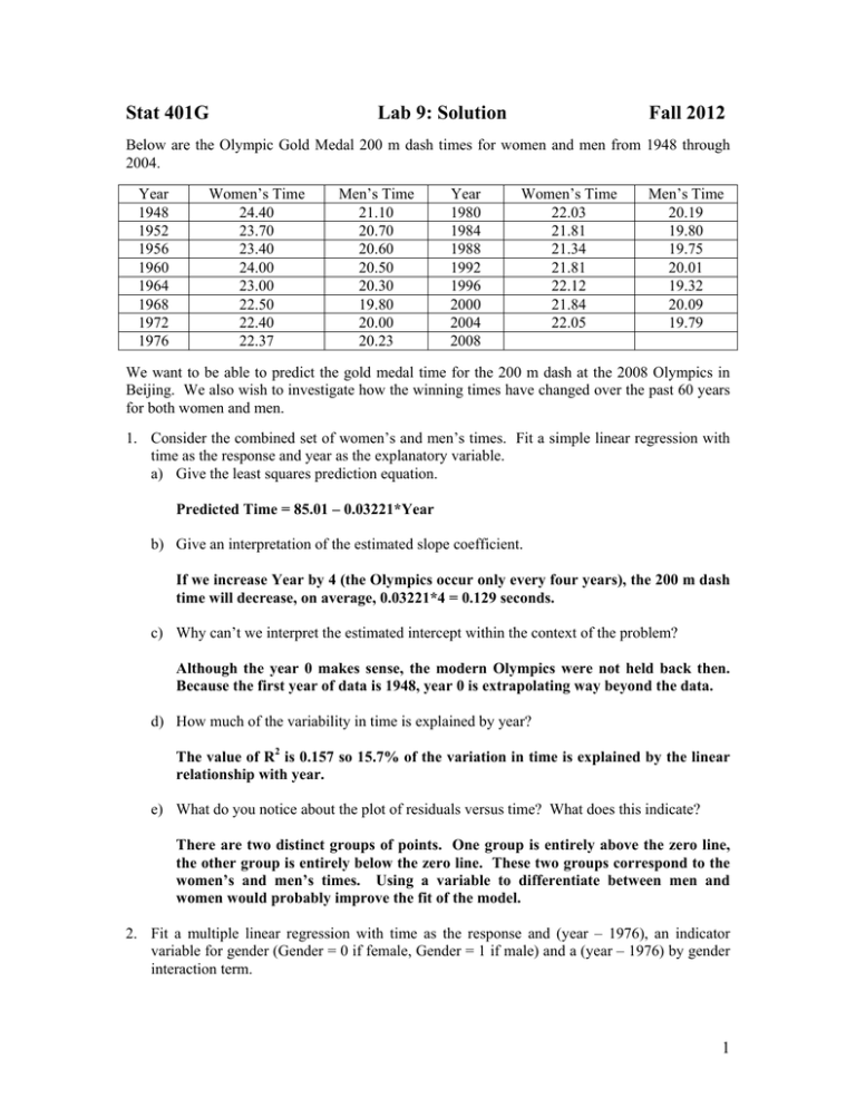
Stat 401G
Lab 9: Solution
Fall 2012
Below are the Olympic Gold Medal 200 m dash times for women and men from 1948 through
2004.
Year
1948
1952
1956
1960
1964
1968
1972
1976
Women’s Time
24.40
23.70
23.40
24.00
23.00
22.50
22.40
22.37
Men’s Time
21.10
20.70
20.60
20.50
20.30
19.80
20.00
20.23
Year
1980
1984
1988
1992
1996
2000
2004
2008
Women’s Time
22.03
21.81
21.34
21.81
22.12
21.84
22.05
Men’s Time
20.19
19.80
19.75
20.01
19.32
20.09
19.79
We want to be able to predict the gold medal time for the 200 m dash at the 2008 Olympics in
Beijing. We also wish to investigate how the winning times have changed over the past 60 years
for both women and men.
1. Consider the combined set of women’s and men’s times. Fit a simple linear regression with
time as the response and year as the explanatory variable.
a) Give the least squares prediction equation.
Predicted Time = 85.01 – 0.03221*Year
b) Give an interpretation of the estimated slope coefficient.
If we increase Year by 4 (the Olympics occur only every four years), the 200 m dash
time will decrease, on average, 0.03221*4 = 0.129 seconds.
c) Why can’t we interpret the estimated intercept within the context of the problem?
Although the year 0 makes sense, the modern Olympics were not held back then.
Because the first year of data is 1948, year 0 is extrapolating way beyond the data.
d) How much of the variability in time is explained by year?
The value of R2 is 0.157 so 15.7% of the variation in time is explained by the linear
relationship with year.
e) What do you notice about the plot of residuals versus time? What does this indicate?
There are two distinct groups of points. One group is entirely above the zero line,
the other group is entirely below the zero line. These two groups correspond to the
women’s and men’s times. Using a variable to differentiate between men and
women would probably improve the fit of the model.
2. Fit a multiple linear regression with time as the response and (year – 1976), an indicator
variable for gender (Gender = 0 if female, Gender = 1 if male) and a (year – 1976) by gender
interaction term.
1
a) How much of the variability in time is explained by this model?
The value of R2 is 0.935 so 93.5% of the variation in time is explained by the
interaction model with (Year – 1976) and Gender.
b) Give the least squares prediction equation for this model.
Predicted Time = 22.585 – 0.0442*(Year – 1976) – 2.439*Gender
+ 0.0240*(Year – 1976)*Gender
c) Interpret each of the estimated parameters within the context of the problem.
In 1976, (Year – 1976) = 0, the predicted 200 m dash time for women (Gender = 0) is
22.585, on average.
Holding Gender constant at 0 (women), a 4 year increase in (Year – 1976) will see a
decrease of 0.0442*4 = 0.177 seconds, on average. That is, the average decrease in
women’s 200 meter dash time from one Olympics to the next is 0.177 seconds.
In 1976, (Year – 1976), men are predicted to be 2.439 seconds faster than women, on
average.
The estimated coefficient for the interaction term (Year – 1976)*Gender is the
difference in the rates of change for men compared to women. On average, men’s
200 m dash times are decreasing at a slower rate than women’s, 0.0240 seconds per
year slower.
d) In 1976, were the predicted times for men and women statistically different? Support
your answer with the appropriate test or confidence interval.
Yes. This is just a test of significance for the estimated slope for Gender. The value
of the test statistic is either t = –17.41 or F = 303.21 with associated P-value < 0.0001.
The small P-value indicates a statistically significant difference between the genders
in 1976.
e) Are women’s and men’s times changing at statistically different rates? Support your
answer with the appropriate test or confidence interval.
Yes. This is just a test of significance for the estimated slope for the interaction
term. The value of the test statistic is either t = 2.96 or F = 8.75 with associated Pvalue of 0.0065. The small P-value indicates that the women’s and men’s times are
changing at different rates from year to year.
f) Predict the winning times for women and men at the 2008 Beijing Olympics. How do
these predictions compare to the actual times of 19.30 for men and 21.74 for women?
Women: Predicted time = 21.17 seconds
Men: Predicted time = 19.50 seconds
The women’s predicted time is too low and the men’s predicted time is a little high.
2
g) Describe the plot of residuals versus year. What does this indicate about the fit of the
model?
There is an indication of a curve in the plot of residuals versus year. Up through
1960 most of the points are above the zero line. From 1964 through 1988 most of the
points are below the zero line. From 1992 through 2004 most of the points are
above the zero line. Adding a quadratic term for year may improve the fit of the
model.
3. Fit a multiple linear regression with time as the response and (year – 1976), Gender,
Gender*(year – 1976), (year – 1976)2, and Gender*(year – 1976)2.
a) How much of the variability in time is explained by this model?
The value of R2 is 0.969 so 96.9% of the variation in time is explained by this model.
b) Does Gender*(Year – 1976)2 add significantly to the model? Support your answer
statistically.
No. The test statistic is either t = a – 1.88 or F = 3.53 with associated P-value of
0.0725. Because the P-value is not small (> 0.05) the Gender*(Year – 1976)2 does not
add significantly to the model with the other four variables in it.
c) What is the “best” model for predicting time? Give the prediction equation.
The “best” model includes the terms; (Year – 1976), Gender, (Year – 1976)*Gender
and (Year – 1976)2.
Predicted Time = 22.313 – 0.0442*(Year – 1976) – 2.4393*Gender +
0.0240*Gender*(Year – 1976) + 0.00091*(Year – 1976)2.
d) Use this “best” model to predict the men’s and women’s 200 m dash times for the 2008
Beijing Olympics. How do these predictions compare to the actual times of 19.30 for
men and 21.74 for women?
Women: Predicted time = 21.83 seconds
Men: Predicted time = 20.16 seconds
The prediction for men is too high but the prediction for women is pretty close.
e) Analyze the residuals for the “best” model. What does this analysis indicate about the
conditions of equal standard deviations, identically and normally distributed errors?
The plots of residuals versus the explanatory variables, Year and Gender, show
relatively equal spreads so the condition of equal standard deviations is probably
met.
The box plot shows a potential outlier at around +0.75. This indicates that the
identically distributed error condition is probably not met.
The histogram is mounded to the left of zero and skewed right. With the exception
of the one large residual, the box plot is fairly symmetric. Most of the points on the
Normal Quantile Plot fall close to the diagonal Normal model line. The normally
distributed error condition could go either way. There is some evidence against it
but that evidence is not that strong.
3