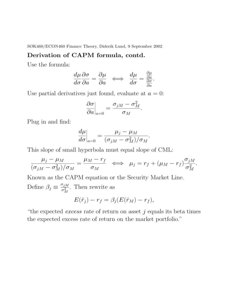
SØK460/ECON460 Finance Theory, Diderik Lund, 9 September 2002
Derivation of CAPM formula, contd.
Use the formula:
dµ ∂σ ∂µ
dµ
=
⇐⇒
=
dσ ∂a ∂a
dσ
∂µ
∂a
∂σ .
∂a
Use partial derivatives just found, evaluate at a = 0:
2
σjM − σM
∂σ .
=
∂a a=0
σM
Plug in and find:
dµ µj − µM
=
2 )/σ .
dσ a=0 (σjM − σM
M
This slope of small hyperbola must equal slope of CML:
µj − µM
µM − r f
=
2 )/σ
(σjM − σM
σM
M
⇐⇒ µj = rf + (µM − rf )
σjM
2 .
σM
Known as the CAPM equation or the Security Market Line.
Define βj ≡
σjM
2 .
σM
Then rewrite as
E(r̃j ) − rf = βj (E(r̃M ) − rf ),
“the expected excess rate of return on asset j equals its beta times
the expected excess rate of return on the market portfolio.”
SØK460/ECON460 Finance Theory, Diderik Lund, 9 September 2002
Illustrating the Security Market Line
µj = rf + βj (µM − rf ).
• All securities are located on the line.
• Also any portfolio of m securities. Show for m = 2:
µp = aµi +(1−a)µj = a[rf +βi(µM −rf )]+(1−a)[rf +βj (µM −rf )]
= rf + [aβi + (1 − a)βj ](µM − rf )


cov(r̃j , r̃M ) 
cov(r̃i, r̃M )
 (µM − rf )
+
(1
−
a)
2
2
σM
σM
cov(ar̃i + (1 − a)r̃j , r̃M )
= rf +
(µM − rf )
2
σM
cov(r̃p, r̃M )
= rf +
(µM − rf ) = rf + βp(µM − rf ).
2
σM
= rf + a
SØK460/ECON460 Finance Theory, Diderik Lund, 9 September 2002
Interpretation of CAPM equation
E(r̃j ) = rf +
σjM
2 (E(r̃M ) − rf ).
σM
Verbal interpretation:
The expected rate of return on any asset depends on only
one characteristic of that asset, namely its rate of return’s
covariance with the rate of return on the market portfolio.
The expected rate of return is equal to the risk free interest rate plus a term which depends on a measure of risk.
(Higher risk means higher expected rate of return.) The
relevant measure of risk is the asset’s beta. This is multiplied with the expected excess rate of return on the market
portfolio.
• Obvious: Does not say what rj will be. Only E(r̃j ).
• Risk measure depends on covariance because the covariance
determines how much that asset will contribute to the risk of
the agent’s portfolio.
• This is true for any agent, since all hold the same risky portfolio.
SØK460/ECON460 Finance Theory, Diderik Lund, 9 September 2002
Interpretation, contd.
• Observe βM = 1.
• Observe βj = ρjM σj /σM .
• May have σj > σM , and ρjM close to 1.
• Thus possible to have βj > 1 for some assets.
• May also have cov(r̃j , r̃M ) < 0, βj < 0.
• Not very common in practice.
• Such assets contribute to reducing σM (when included in M).
• Valuable to investors, thus high value at t = 0, thus low expected rate of return.
SØK460/ECON460 Finance Theory, Diderik Lund, 9 September 2002
Avoid confusion
• Do not confuse the following two:
• The Capital Market Line:
– Efficient set given 1 risk free and n risky assets.
– Relevant for choice between alternative portfolios.
– Drawn in (σp, µp) diagram.
– A ray starting at (0, rf ) in that diagram.
• The Security Market Line:
– Location of all traded assets in equilibrium.
– Also location of any portfolio of these assets.
– Not relevant for choice between assets which are already
traded, so that equilibrium prices are observable.
– But relevant if equilibrium price at t = 0 is unknown.
– Drawn in (βj , µj ) diagram.
– A line through (0, rf ) in that diagram.
SØK460/ECON460 Finance Theory, Diderik Lund, 9 September 2002
Other forms of the CAPM equation
Remember: 1 + r̃j = p̃j1/pj0. Rewrite:


µM − r f
E(p̃j1)
 p̃j1



r̃
− 1 = rf +
cov
−
1,
M
2
pj0
σM
pj0


p̃j1
E(p̃j1)

,
= 1 + rf + λ cov 
, r̃M 
⇐⇒
pj0
pj0
2
with λ defined as (µM − rf )/σM
.
1
pj0
is deterministic, and can be factored out of the covariance. Multiply both sides by
pj0
1 + rf
and rearrange terms to get
pj0 =
1
[E(p˜j1) − λ cov(p̃j1, r̃M )] .
1 + rf
Expression in square bracket is called the certainty equivalent (in
the CAPM sense) of p̃j1. Price today is present value of expression,
just as if that would be received with certainty one period into the
future. Not what is called certainty equivalent in expected utility
theory.
SØK460/ECON460 Finance Theory, Diderik Lund, 9 September 2002
Other forms of the CAPM expression, contd.
Can also rewrite as
pj0 =
E(p̃j1)
.
1 + rf + λ cov(r̃j , r̃M )
(Prove yourself how to arrive at this!)
• Like previous form: pj0 on left-hand side.
• But here: Right-hand side is “expected present value.”
• However: Risk-adjusted discount rate, RADR.
• Obtained by adding something to rf .
• Risk-adjustment again depends on λ and covariance.
• Observe difference in covariance expressions!
• Previously: cov(p̃j1, r̃M ).
• Now: cov(r̃j , r̃M ) ≡ cov(p̃j1/pj0, r̃M ).
• If need to solve for pj0, the formula on top of this page is less
useful: It has pj0 also on right-hand side, “hidden” in covariance
term.
• Use instead expression on previous page.
SØK460/ECON460 Finance Theory, Diderik Lund, 9 September 2002
CAPM: Implications, applications
• For a portfolio: Variance the relevant risk measure.
• For each security: Covariance with r̃M the relevant r. m.
• Reason: Covariance measures contribution to portfolio variance.
• Generally: Covariance with each agent’s marginal utility.
• But when mean-var preferences: Covariance with agent’s wealth.
• In equilibrium: All have same risky portfolio (composition).
• Thus covariance with r̃M relevant for everyone.
• Implication: Adding noise does not matter:
• Suppose p̃h1 = p̃j1 + ε̃, where E(ε̃) = 0 and ε̃ is stochastically
independent of (p̃j1, r̃M ). Can show ph0 = pj0:
ph0 =
=
1
[E(p̃j1 + ε̃) − λ cov(p̃j1 + ε̃, r̃M )]
1 + rf
1
[E(p̃j1) + E(ε̃) − λ[cov(p̃j1, r̃M ) + cov(ε̃, r̃M )]] = pj0.
1 + rf
• At this point: Do not get confused by ρjM .
• Common confusion: Since σjM = ρjM σj σM , some believe that
a higher σj leads to a higher σjM .
• Have just shown a case where this is not true; instead:
ρhM =
σhM
σjM
σjM
=
<
= ρjM .
σhσM
σhσM
σj σM
SØK460/ECON460 Finance Theory, Diderik Lund, 9 September 2002
CAPM terminology: Systematic vs. unsystematic risk
Define ε̃j through the equation
r̃j = rf + βj [r̃M − rf ] + ε̃j .
Then the CAPM equation
E(r̃j ) = rf + βj [E(r̃M ) − rf ]
implies that E(ε̃j ) = 0, and that
2
cov(ε̃j , r̃M ) = cov(r̃j , r̃M ) − βj var(r̃M ) = σjM − βj σM
= 0.
This allows us to split σj2 in two parts:
2
var(r̃j ) ≡ σj2 = βj2σM
+ σε2j = βj σjM + σε2j .
First term called systematic risk. This is reflected in the market
valuation. (More general term: Relevant risk or covariance risk.)
Second term called unsystematic risk. As we have seen, it is not
reflected in market valuation. (More general term: Irrelevant risk.)
The sum of the two called total risk or variance risk. This is
relevant for portfolios, evaluated for being the total wealth of someone, but not for individual securities, to be combined with other
securities in portfolios.
SØK460/ECON460 Finance Theory, Diderik Lund, 9 September 2002
Valuation of firms, value additivity
pi0 =
1
[E(p̃i1) − λ cov(p̃i1, r̃M )] ≡ V (p̃i1),
1 + rf
defines valuation function V (), given some rf , r̃M .
• p̃i1 is value of share at t = 1, including dividends.
• Consider firm financed 100% by equity (no debt).
• Firm’s net cash flow at t = 1 goes to shareholders.
• Plug in that net cash flow instead of p̃i1.
• Then formula gives value of all shares in firm.
• What if p̃i1 = ap̃j1 + bp̃k1? (a > 0, b > 0 constants.)
• Linearity of E() and cov() implies pi0 = apj0 + bpk0:
pi0 =
=
=
1
[E(p̃i1) − λ cov(p̃i1, r̃M )]
1 + rf
1
[E(ap̃j1 + bp̃k1) − λ cov(ap̃j1 + bp̃k1, r̃M )]
1 + rf
1
[aE(p̃j1) + bE(p̃k1) − λ[a cov(p̃j1, r̃M ) + b cov(p̃k1, r̃M )]]
1 + rf
= apj0 + bpk0.
• Diversification is no justification for mergers.
• Diversification can be done by shareholders.
SØK460/ECON460 Finance Theory, Diderik Lund, 9 September 2002
Investment project’s rate of return
• Consider (potential) real investment project:
– Outlay I at t = 0.
– Revenue p̃I1 at t = 1.
• Project value? Should project be undertaken?
• Assume 100% equity financed. (Assume separate firm?)
• Project’s rate of return is (p̃I1 − I)/I.
• If use of restricted technology or resources: No reason for SML
equation to hold for this rate of return.
• May earn above-normal expected rate of return.
• However: Valuation of p̃I1 possible:
pI0 = V (p̃I1) =
1
[E(p̃I1) − λ cov(p̃I1, r̃M )]
1 + rf
defines pI0 independently of I.
• If pI0 > I, undertake project. Net value pI0 − I.
• If pI0 < I, drop project. Net value of opportunity is 0. Net
value of having to undertake project is pI0 − I, negative.
• Competition and free entry ⇒ pI0 = I.
SØK460/ECON460 Finance Theory, Diderik Lund, 9 September 2002
Project valuation, contd.
• If claim to p̃I1 costs pI0, this is equilibrium price.
• Project is then on security market line (SML).
• If project available at different cost I: Not at SML.
Project’s βk , must satisfy the equation
E(
p̃I1
) = 1 + rf + [µM − rf ]βk
pI0
p̃I1
2
, r̃M )/σM
.
pI0
Expressed in terms of exogenous variables (eliminating pI0) this
becomes
(1 + rf )
βk = 2 E(p̃ )
,
σM cov(p̃ I1,r̃ ) − µM + rf
= 1 + rf + [µM − rf ] cov(
I1 M
independent of I. Only if I = pI0 = V (p̃I1), will the project rate
of return p̃I1/I − 1 satisfy the CAPM equation with βk .