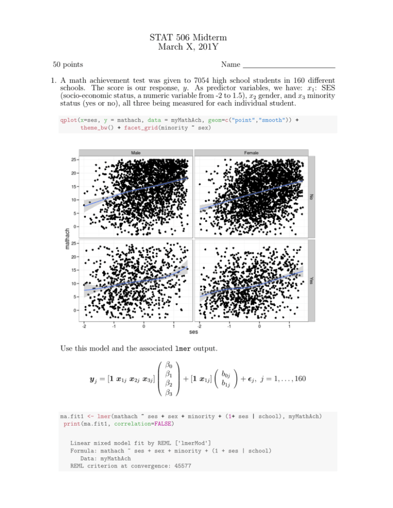
STAT 506 Midterm
March X, 201Y
50 points
Name
1. A math achievement test was given to 7054 high school students in 160 different
schools. The score is our response, y. As predictor variables, we have: x1 : SES
(socio-economic status, a numeric variable from -2 to 1.5), x2 gender, and x3 minority
status (yes or no), all three being measured for each individual student.
qplot(x=ses, y = mathach, data = myMathAch, geom=c("point","smooth")) +
theme_bw() + facet_grid(minority ~ sex)
Use this model and the associated lmer output.

y j = [1


x1j x2j x3j ] 

β0
β1
β2
β3



 + [1

x1j ]
b0j
b1j
!
+ j , j = 1, . . . , 160
ma.fit1 <- lmer(mathach ~ ses + sex + minority + (1+ ses | school), myMathAch)
print(ma.fit1, correlation=FALSE)
Linear mixed model fit by REML ['lmerMod']
Formula: mathach ~ ses + sex + minority + (1 + ses | school)
Data: myMathAch
REML criterion at convergence: 45577
Exam 1 Stat 506 Page 2
Random effects:
Groups
Name
Std.Dev. Corr
school
(Intercept) 1.914
ses
0.574
-0.41
Residual
5.994
Number of obs: 7054, groups: school, 160
Fixed Effects:
(Intercept)
ses
sexFemale minorityYes
14.16
2.11
-1.20
-2.99
(a) Interpret estimated population effects for ses, minority, and sex (skip the intercept). Give the estimated size, sign, and the strength of evidence for each
being nonzero. Explain in terms of this situation, not just in general platitudes.
(10pts)
(b) Write out the estimated distribution of
b0j
b1j
!
. Plug in the estimates from the
output.
(5 pts)
(c) Ses appears in the model twice. Explain the difference in interpretation between
the two ses outputs.
(4 pts)
(d) Let y 1 be the vector of 15 math achievement scores for the first school (labeled
8367 below).
xtable(head(ranef(ma.fit1)[["school"]]))
8367
8854
4458
5762
6990
5815
(Intercept)
-4.98
-4.99
-2.38
-2.83
-2.84
-2.42
ses
0.46
0.65
0.23
0.36
0.14
0.37
i. Write down its predicted mean vector (based on x1j , x2j , x3j which you
don’t have access to for this exam, just use them as symbols) plugging in
the estimates from the output.
(5 pts)
ii. What is the estimated variance-covariance of y 1 ? (Hint: avoid rewriting
things you already explained above by giving them a label above and just
using that here.)
(5 pts)
(e) If we did the same analysis in SAS PROC MIXED:
i. How would the fixed effects SAS reports differ from those of R?
(3 pts)
ii. How would the random effects SAS reports differ from those of R? (3 pts)
(f) Two other models were considered. Explain how they differ and which you
prefer based on the following output.
(6 pts)
Exam 1 Stat 506 Page 3
ma.fit2 <- lmer(mathach ~ ses * minority + sex + (1+ ses | school), myMathAch)
ma.fit3 <- lmer(mathach ~ ses * minority + ses * sex + (1+ ses | school), myMath
xtable(AIC(ma.fit1,ma.fit2,ma.fit3))
ma.fit1
ma.fit2
ma.fit3
df
AIC
8.00 45593.02
9.00 45580.31
10.00 45579.78
2. Consider a comparison of two curricula (A and B) for teaching intro stats to college
students. Students will register for a section of the class which fits their schedule not
knowing if the section will be taught using the A or the B curriculum.
(a) How will this design allow for causal inference? Explain any necessary assumptions.
(5
pts)
(b) Curriculum B requires two 75 minute meeting times each week, but A will
be taught in three 50 minute sessions. Discuss in terms of imbalance and/or
overlap. What further assumption(s) is(are) required?
(4 pts)