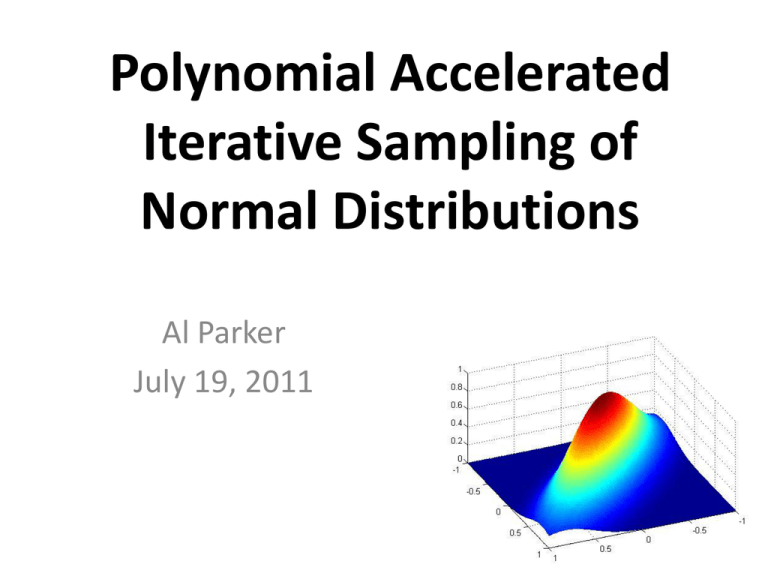
Polynomial Accelerated
Iterative Sampling of
Normal Distributions
Al Parker
July 19, 2011
Acknowledgements
• Colin Fox, Physics,
University of Otago
• New Zealand Institute of Mathematics,
University of Auckland
• Center for Biofilm Engineering,
, Bozeman
The multivariate Gaussian distribution
1
 1

T
1
N ( , )  n
exp   ( y   )  ( y   ) 
1/ 2
2 det( )
 2

How to sample from a Gaussian N(µ,Σ)?
• Sample z ~ N(0,I)
y = Σ1/2 z+ µ
~ N(µ,Σ)
The problem
• To generate a sample y = Σ1/2 z+ µ ~ N(µ,Σ),
how to calculate the factorization Σ =Σ1/2(Σ1/2)T ?
• Σ1/2 = WΛ1/2 by eigen-decomposition, 10/3n3 flops
• Σ1/2 = C by Cholesky factorization, 1/3n3 flops
LARGE
For
Gaussians (n>105, eg in image analysis
and global data sets), these factorizations are not possible
• n3 is computationally TOO EXPENSIVE
• storing an n x n matrix requires TOO MUCH MEMORY
Some solutions
Work with sparse precision matrix Σ-1 models (Rue, 2001)
Circulant embeddings (Gneiting et al, 2005)
Iterative methods:
• Advantages:
– COST: n2 flops per iteration
– MEMORY: Only vectors of size n x 1 need be stored
• Disadvantages:
– If the method runs for n iterations, then there is no cost
savings over a direct method
What iterative samplers are available?
Sampling y ~ N(0,A-1):
Gibbs
Chebyshev-Gibbs
Lanczos
Solving Ax=b:
Gauss-Seidel
Chebyshev-GS
CG-Lanczos
What’s the link to Ax=b?
Solving Ax=b is equivalent to minimizing an ndimensional quadratic (when A is spd)
1 T
f ( x)  x Ax  bT x
2
f ( x)  b  Ax
A Gaussian is sufficiently specified by the same quadratic
(with A= Σ-1and b=Aμ):
1
 1

T
1
N ( , )  n
exp

(
y


)

(
y


)


1/ 2
2 det( )
 2

CG-Lanczos solver and sampler
CG-Lanczos estimates:
• a solution to Ax=b
• eigenvectors of A
in a k-dimensional Krylov space
CG sampler produces:
• y ~ N(0, Σy ≈ A-1)
• Ay ~ N(0, AΣyA ≈ A)
with accurate covariances in the same
k-dimensional Krylov space
Schneider and Willsky, 2001
Parker and Fox, 2011
CG-Lanczos solver in finite precision
The CG-Lanczos search directions span a Krylov space much
smaller than the full space of interest.
CG is still guaranteed to find a solution to Ax = b …
Lanczos eigensolver will only estimate a few of the
eigenvectors of A …
CG sampler produces
y ~ N(0, Σy ≈ A-1)
Ay ~ N(0, AΣyA ≈ A)
with accurate covariances …
… in the eigenspaces corresponding
to the well separated eigenvalues
of A that are contained in the
k-dimensional Krylov space
Example: N(0,A) over a 1D domain
A=
covariance matrix
eigenvalues of A
Only 8 eigenvectors
(corresponding to the 8 largest
eigenvalues)
are sampled (and estimated) by
the CG sampler
Example: N(0,A) over a 1D domain
Ay ~ N(0, A)
Cholesky sample
CG sample
λ -(k+1) ≤ ||A - Var(AyCG)||2 ≤ λ -(k+1) + ε
Example: 104 Laplacian over a 2D domain
A(100:100) =
precision matrix
A-1(100:100) =
covariance matrix
Example: 104 Laplacian over a 2D domain
eigenvalues of A-1
35 eigenvectors
are sampled
(and estimated)
by the CG sampler.
Example: 104 Laplacian over a 2D domain
y ~ N(0, A-1)
Cholesky sample
CG sample
trace(Var(yCG)) / trace(A-1) = 0.80
How about an iterative sampler from
LARGE Gaussians
that is guaranteed to converge for arbitrary
covariance or precision matrices?
Could apply
re-orthogonalization
to maintain an
orthogonal
Krylov basis,
but this is expensive
(Schneider and Willsky, 2001)
Gibbs: an iterative sampler
Gibbs sampling from N(µ,Σ) starting from (0,0)
Gibbs: an iterative sampler of
N(0,A) and N(0, A-1 )
Let A=Σ or A= Σ-1
1. Split A into D=diag(A), L=lower(A), LT=upper(A)
2. Sample z ~ N(0,I)
3. Take conditional samples in each coordinate
direction, so that a full sweep of all n coordinates is
yk =-D-1 L yk - D-1 LT yk-1 + D-1/2 z
yk converges in distribution geometrically to N(0,A-1)
E(yk)= Gk E(y0)
Var(yk) = A-1 - Gk (A-1 - Var(y0))GkT
Ayk converges in distribution geometrically to N(0,A)
Goodman and Sokal, 1989
Gauss-Siedel Linear Solve of Ax=b
1. Split A into D=diag(A), L=lower (A), LT=upper(A)
2. Minimize the quadratic f(x) in each coordinate
direction, so that a full sweep of all n coordinates
is
xk =-D-1 L xk - D-1 LT xk-1 + D-1 b
xk converges geometrically A-1b
(xk - A-1b) = Gk( x0 - A-1b)
where ρ(G) < 1
Theorem: A Gibbs sampler is a
Gauss Siedel linear solver
Proof:
• A Gibbs sampler is
yk =-D-1 L yk - D-1 LT yk-1 + D-1/2 z
• A Gauss-Siedel linear solve of Ax=b is
xk =-D-1 L xk - D-1 LT xk-1 + D-1 b
Gauss Siedel is a Stationary Linear Solver
• A Gauss-Siedel linear solve of Ax=b is
xk =-D-1 L xk - D-1 LT xk-1 + D-1 b
• Gauss Siedel can be written as
M xk = N xk-1 + b
where M = D + L and N = D - LT , A = M – N,
the general form of a stationary linear solver
Stationary Samplers from
Stationary Solvers
Solving Ax=b:
1. Split A=M-N, where M is invertible
2. Iterate Mxk = N xk-1 + b
xk  A-1b if ρ(G=M-1N)< 1
Need to be able to
easily solve M y = u
Need to be able to
easily sample ck-1
Sampling from N(0,A) and N(0,A-1):
1. Split A=M-N, where M is invertible
2. Iterate Myk = N yk-1 + ck-1
where ck-1 ~ N(0, MT + N)
yk  N(0,A-1) if ρ(G=M-1N)< 1
Ayk  N(0,A) if ρ(G=M-1N)< 1
How to sample
ck-1 ~ N(0, MT + N) ?
M
Var(ck-1) = MT + N convergence
0<w<
2/p(A)
2/w I - A
Richardson
1/w I
Jacobi
D
2D - A
GS/Gibbs
D+L
D
always
SOR/BF
1/w D + L
0<w<2
SSOR/REGS
w/(2-w) MSOR D MTSOR
(2-w)/w D
w/(2 - w)
(MSORD-1 MTSOR +
NSOR D-1 NTSOR)
0<w<2
Theorem:
Stat Linear Solver converges
iff
Stat Sampler converges
Proof: They have the same iteration operator G=M-1N:
For linear solves:
xk = Gxk-1 + M-1 b
so that (xk - A-1b) = Gk( x0 - A-1b)
For sampling G=M-1N:
yk = Gyk-1 + M-1 ck-1
E(yk)= Gk E(y0)
Var(yk) = A-1 - Gk (A-1 - Var(y0))GkT
Proof for SOR given by Adler 1981; Barone and Frigessi, 1990; Amit and Grenander 1991. SSOR/REGS:
Roberts and Sahu 1997.
Acceleration schemes for
stationary linear solvers can be used to
accelerate stationary samplers
Polynomial acceleration of a stationary solver of
Ax=b is
1. Split A = M - N
2. xk+1 = (1- vk) xk-1 + vk xk + vk uk M-1 (b-A xk)
which replaces
(xk - A-1b) = Gk(x0 - A-1b) = (I - (I - G))k(x0 - A-1b)
with a different kth order polynomial with smaller spectral radius
(xk - A-1b) = Pk(I-G)(x0 - A-1b)
Some polynomial accelerated linear solvers …
xk+1 = (1- vk) xk-1 + vk xk + vk uk M-1 (b-A xk)
Gauss-Seidel
vk = uk = 1
Chebyshev-GS
vk and uk are
functions of
the 2 extreme
eigenvalues of
G
CG-Lanczos
vk , uk are
functions of
the residuals
b-Axk
Some polynomial accelerated linear solvers …
(xk - A-1b) = Pk(I-G)(x0 - A-1b)
Gauss-Seidel
Pk(I-G) = Gk
Chebyshev-GS
Pk(I-G)
is the kth order
Chebyshev polynomial
(which has the
smallest maximum
between the two
eigenvalues).
CG-Lanczos
Pk(I-G)
is the kth order
Lanczos
polynomial
How to find polynomial accelerated samplers?
yk+1 = (1- vk) yk-1 + vk yk + vk uk M-1 (ck -A yk)
ck ~ N(0, (2-vk)/vk ( (2 – uk)/ uk M + N)
Gibbs
vk = uk = 1
Chebyshev-Gibbs
vk and uk are
functions of
the 2 extreme
eigenvalues of
G
Lanczos
vk , uk are
functions of
the residuals
b-Axk
Convergence of polynomial accelerated samplers
E(yk)=
Var(yk) = A-1 -
Pk(I-G) E(y0)
Pk(I-G) (A-1 - Var(y0))
Gibbs
Pk(I-G) = Gk
Theorem:
The sampler converges
if the solver converges
Fox and Parker, 2011
Pk(I-G)T
Chebyshev-Gibbs
Pk(I-G)
is the kth order
Chebyshev polynomial
(which has the
smallest maximum
between the two
eigenvalues).
(A-1 - Var(yk))v = 0
(A - Var(Ayk))v = 0
for any Krylov vector v
CG-Lanczos
Pk(I-G)
is the kth order
Lanczos
polynomial
Chebyshev accelerated Gibbs sampler
of N(0,
Covariance
matrix
convergence
||A-1 – Var(yk)||2
-1
) in 100D
Chebyshev accelerated Gibbs can be adapted
to sample under
positivity constraints
One extremely effective sampler for
LARGE Gaussians
Use a combination of the ideas presented:
• Use the CG sampler to generate samples and
estimates of the extreme eigenvalues of G.
• Seed these samples and extreme eigenvalues
into a Chebyshev accelerated SSOR sampler
Conclusions
Common techniques from numerical linear
algebra can be used to sample from Gaussians
• Cholesky factorization (precise but expensive)
• Any stationary linear solver can be used as a
stationary sampler (inexpensive but with geometric convergence)
• Polynomial accelerated Samplers
– Chebyshev (precise and inexpensive)
– CG (precise in a some eigenspaces and inexpensive)