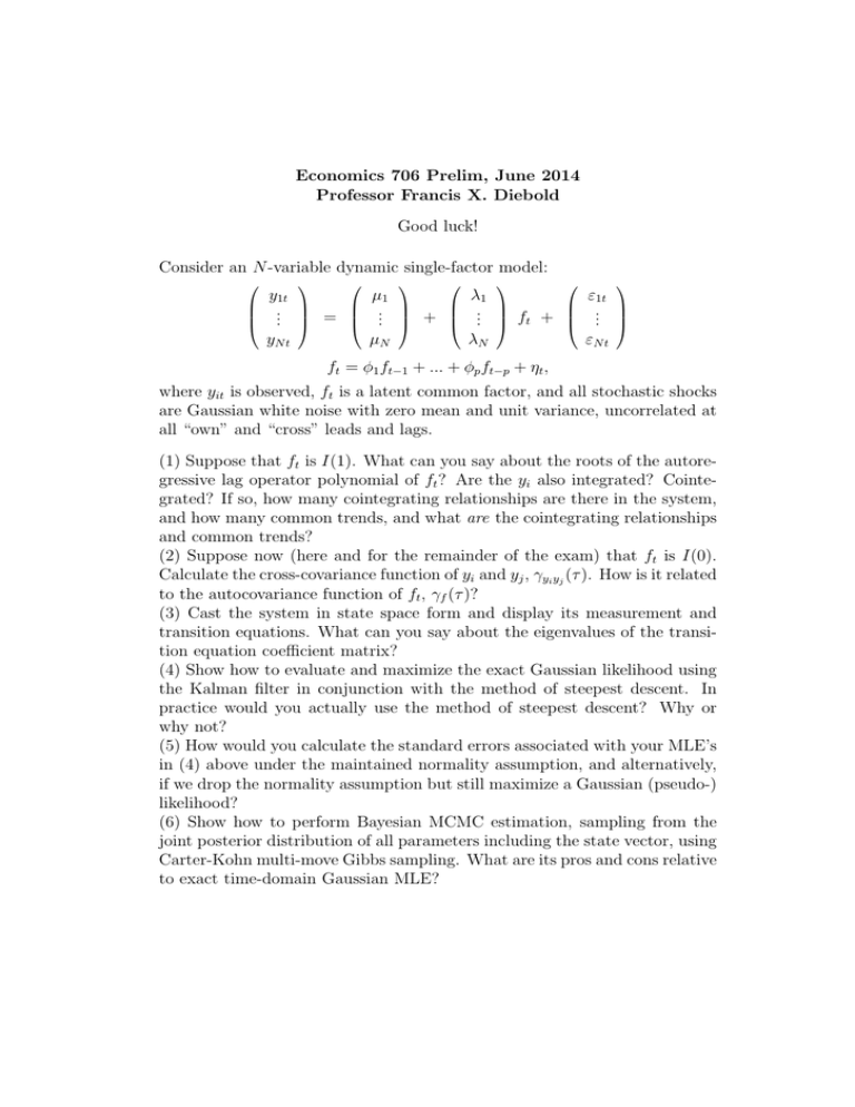
Economics 706 Prelim, June 2014
Professor Francis X. Diebold
Good luck!
Consider an N -variable dynamic single-factor model:



y1t

 . 
 .  = 

 . 
yN t


µ1

.. 

. 
 + 
µN



ε1t
λ1


.. 
 ft +  .. 
. 
 . 
εN t
λN
ft = φ1 ft−1 + ... + φp ft−p + ηt ,
where yit is observed, ft is a latent common factor, and all stochastic shocks
are Gaussian white noise with zero mean and unit variance, uncorrelated at
all “own” and “cross” leads and lags.
(1) Suppose that ft is I(1). What can you say about the roots of the autoregressive lag operator polynomial of ft ? Are the yi also integrated? Cointegrated? If so, how many cointegrating relationships are there in the system,
and how many common trends, and what are the cointegrating relationships
and common trends?
(2) Suppose now (here and for the remainder of the exam) that ft is I(0).
Calculate the cross-covariance function of yi and yj , γyi yj (τ ). How is it related
to the autocovariance function of ft , γf (τ )?
(3) Cast the system in state space form and display its measurement and
transition equations. What can you say about the eigenvalues of the transition equation coefficient matrix?
(4) Show how to evaluate and maximize the exact Gaussian likelihood using
the Kalman filter in conjunction with the method of steepest descent. In
practice would you actually use the method of steepest descent? Why or
why not?
(5) How would you calculate the standard errors associated with your MLE’s
in (4) above under the maintained normality assumption, and alternatively,
if we drop the normality assumption but still maximize a Gaussian (pseudo-)
likelihood?
(6) Show how to perform Bayesian MCMC estimation, sampling from the
joint posterior distribution of all parameters including the state vector, using
Carter-Kohn multi-move Gibbs sampling. What are its pros and cons relative
to exact time-domain Gaussian MLE?