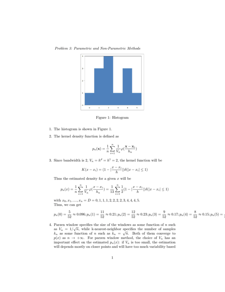
Problem 3: Parametric and Non-Parametric Methods
Figure 1: Histogram
1. The histogram is shown in Figure 1.
2. The kernel density function is defined as
n
pn (x) =
1X 1
x − xi
ϕ(
)
n i=1 Vn
hn
3. Since bandwidth is 2, Vn = hd = h1 = 2, the kernel function will be
K(x − xi ) = (1 − |
x − xi
|)δ(|x − xi | ≤ 1)
h
Thus the estimated density for a given x will be
n
pn (x) =
n
1X 1
x − xi
x − xi
1 X1
ϕ(
)=
(1 − |
|)δ(|x − xi | ≤ 1)
n i=1 Vn
hn
13 i=1 2
h
with x0 , x1 , ...., xn = D = 0, 1, 1, 1, 2, 2, 2, 2, 3, 4, 4, 4, 5.
Thus, we can get
pn (0) =
5
11
12
9
8
≈ 0.096; pn (1) =
≈ 0.21; pn (2) =
≈ 0.23; pn (3) =
≈ 0.17; pn (4) =
≈ 0.15; pn (5) =
52
52
52
52
52
5
4. Parzen window
√ specifies the size of the windows as some function of n such
as Vn = 1/ n, while k-nearest-neighbor √
specifies the number of samples
kn as some function of n such as kn = n. Both of them converge to
p(x) as n → +∞. For parzen window method, the choice of Vn has an
important effect on the estimated pn (x): if Vn is too small, the estimation
will depends mostly on closer points and will have too much variability based
1
on a limited number of training samples (over-training); if Vn is too large,
the estimation will be an average over a large range of nearby samples, and
will loss some details of p(x). By specifying the number of samples, kNN
methods circumvent this problem by making the window size a function of
the actual training data. If the density is higher around a particular x,
the corresponding Vn will be smaller. This means if we have more samples
around x, we will use smaller window size to capture more details around x.
If the density is lower around x, the corresponding Vn will be larger, which
means less samples can only give us an estimation of a larger scale and cannot
recover many details.
5. If assume the density is a Gaussian, the maximum likelihood estimate of the
Gaussian parameters µ, σ 2 is:
n
µ̂ =
1X
xi ≈ 2.38
n i=1
n
σ̂ 2 =
1X
(xi − µ̂)2 ≈ 2.08
n i=1
The unbiased result is
n
2
σ̂unbias
=
1 X
(xi − µ̂)2 ≈ 2.26
n − 1 i=1
6. Histogram captures the density in a discrete way and can have large errors
around boundaries of bins. The triangle-kernel better captured the density with a smoother representation. Although Gaussian estimation is also
smooth, it cannot capture the data samples very well. That’s because it
assumed Gaussian distribution of the samples, while the given sample data
doesn’t fit into a Gaussian distribution. The triangular-kernel best captured
the data and I would choose this one to estimate the distribution of this
particular data set.
2