18.S096: Homework Problem Set 1 (revised)
Topics in Mathematics of Data Science (Fall 2015)
Afonso S. Bandeira
Due on October 6, 2015
Extended to: October 8, 2015
This homework problem set is due on October 6, at the start of class
Try not to look up the answers, you’ll learn much more if you try to
think about the problems without looking up the solutions.
You can work in groups but each student must write his/her own
solution based on his/her own understanding of the problem.
If you need to impose extra conditions on a problem to make it easier,
state explicitly that you have done so. Solutions where extra conditions
were assumed will also be graded (probably scored as a partial answer).
1.1
Linear Algebra
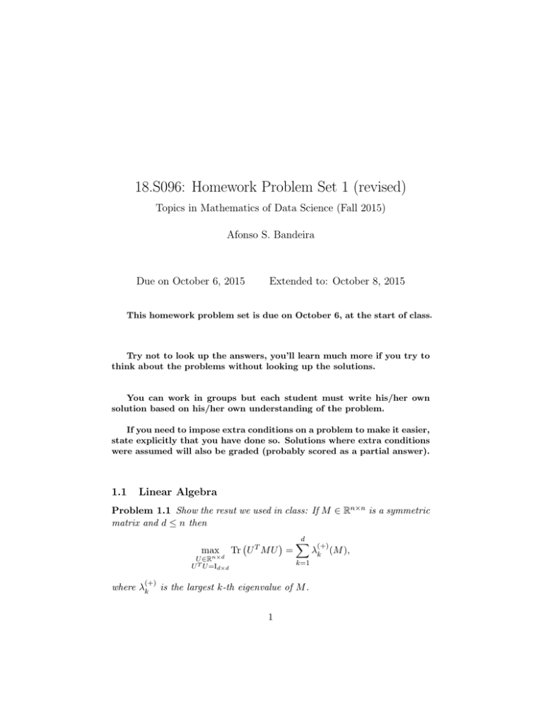
Problem 1.1 Show the resut we used in class: If M ∈ Rn×n is a symmetric
matrix and d ≤ n then
max
U ∈Rn×d
U T U =Id×d
(+)
where λk
d
X
(+)
Tr U T M U =
λk (M ),
k=1
is the largest k-th eigenvalue of M .
1
1.2
Estimators
Problem 1.2 Given x1 , · · · , xn i.i.d. samples from a distribution X with
mean µ and covariance Σ, show that
n
µn =
1X
xk ,
n
n
and
k=1
Σn =
1 X
(xk − µn ) (xk − µn )T ,
n−1
k=1
are unbiased estimators for µ and Σ, i.e., show that E [µn ] = µ and E [Σn ] =
Σ.
1.3
Random Matrices
Recall the definition of a standard gaussian Wigner Matrix W : a symmetric
random matrix W ∈ Rn×n whose diagonal and upper-diagonal entries are
independent Wii ∼ N (0, 2) and, for i < j, Wij ∼ N (0, 1). This random matrix emsemble is invariant under orthogonal conjugation: U T W U ∼ W for
any U ∈ O(n). Also, the distribution of the eigenvalues of √1n W converges
to the so-called semicircular law with support [−2, 2]
p
dSC(x) = 4 − x2 1[−2,2] (x).
(try it in MATLAB® draw an histogram of the distribution of the eigenvalues
of √1n W for, say n = 500.)
In the next problem, you will show that the largest eigenvalue of √1n W
has expected value at most 2.1 For that, we will make use of Slepian’s
Comparison Lemma.
Slepian’s Comparison Lemma is a crucial tool to compare Gaussian Processes. A Gaussian process is a family of gaussian random variables indexed
by some set T , more precisely is a family of gaussian random variables
{Xt }t∈T (if T is finite this is simply a gaussian vector). Given a gaussian process Xt , a particular quantity of interest is E [maxt∈T Xt ]. Intuitively, if we
have two Gaussian processes Xt and
Y2 t withmean
zero E [Xt ] = E [Yt ] = 0,
2
for all t ∈ T and same variances E Xt = E Yt then the process that has
the “least correlations” should have a larger maximum (think the maximum
entry of vector with i.i.d. gaussian entries versus one always with the same
1
Note that, a priori, there could be a very large eigenvalue and it would still not
contradict the semicircular law, since it does not predict what happens to a vanishing
fraction of the eigenvalues.
2
gaussian entry). A simple version of Slepian’s Lemma makes this intuition
precise:2
In the conditions above, if for all t1 , t2 ∈ T
E [Xt1 Xt2 ] ≤ E [Yt1 Yt2 ] ,
then
E max Xt ≥ E max Yt .
t∈T
t∈T
A slightly more general version of it asks that the two Gaussian processes Xt and Yt have mean zero E [Xt ] = E [Yt ] = 0, for all t ∈ T but not
necessarily the same variances. In that case it says that: If or all t1 , t2 ∈ T
E [Xt1 − Xt2 ]2 ≥ E [Yt1 − Yt2 ]2 ,
then
E max Xt
t∈T
(1)
≥ E max Yt .
t∈T
Problem 1.3 We will use Slepian’s Comparison Lemma to show that
√
Eλmax (W ) ≤ 2 n.
1. Note that
λmax (W ) =
max
v: kvk2 =1
v T W v,
which means that, if we take for unit-norm v, Yv := v T W v we have
that
λmax (W ) = E max Yv ,
v∈Sn−1
2. Use Slepian to compare Yv with 2Xv defined as
Xv = v T g,
where g ∼ N (0, In×n )
3. Use Jensen’s inequality to upperbound E [maxv∈Sn−1 Xv ].
2
Although intuitive in some sense, this is a delicate statement about Gaussian random
variables, it turns out not to hold for other distributions.
3
Problem 1.4 In this problem you’ll derive the limit of the largest eigenvalue
of a rank 1 perturbation of a Wigner matrix.
For this problem, you don’t have to justify all of the steps rigorously. You can use the same level of rigor that was used in
class to derive the analogue result for sample covariance matrices. Deriving this phenomena rigorously would take considerably
more work and is outside of the scope of this homework.
Consider the matrix M = √1n W + βvv T for kv k2 = 1 and W a standard Gaussian Wigner matrix. The purpose of this homework problem is to
understand the behavior of λmax (M ). Because W is invariant to orthogonal
conjugation we can focus on understanding
1
T
λmax √ W + βe1 e1 .
n
Use the same techniques as used in class to derive the behavior of this
quantity.
R 2 √4−x2
(Hint: at some point, you’ll probably have to integrate −2 y−x
dx. You
p
R 2 √4−x2
can use the fact that, for y > 2, −2 y−x dx = π y − y 2 − 4 (you can
also use an integrator software, such as Mathematica, for this).
1.4
Diffusion Maps and other embeddings
Problem 1.5 The ring graph on n nodes is a graph where node 1 < k <
n is connected to node k − 1 and k + 1 and node 1 is connected to node
n. Derive the two-dimensional diffusion map embedding for the ring graph
(if the eigenvectors are complex valued, try creating real valued ones using
multiplicity of the eigenvalues). Is it a reasonable embedding of this graph
in two dimensions?
Problem 1.6 (Multidimensional Scaling
Revised ) Suppose you want
to represent n data points in Rd and all you are given is estimates for their
Euclidean distances δij ≈ kxi − xj k22 . Multiimensional scaling attempts to
find an d dimensions that agrees, as much as possible, with these estimates.
Organizing X = [x1 , . . . , xn ] and consider the matrix ∆ whose entries are
δij .
1. Show that, if δij = kxi − xj k22 then there is a choice of xi (note that
the solution is not unique, as a translation of the points will preserve
the pairwise distances, e.g.) for which
1
X T X = − H∆H,
2
4
where H = I − n1 11T .
2. If the goal is to find points in Rd , how would you do it (keep part 1 of
the question in mind)?
(The procedure you have just derived is known as Multidimensional Scaling)
This motivates a way to embed a graph in d dimensions. Given two nodes
we take δij to be the square of some natural distance on a graph such as, for
example, the geodesic distance (the distance of the shortest path between the
nodes) and then use the ideas above to find an embedding in Rd for which
Euclidean distances most resemble geodesic distances on the graph. This is
the motivation behind a dimension reduction technique called ISOMAP (J.
B. Tenenbaum, V. de Silva, and J. C. Langford, Science 2000).
5
MIT OpenCourseWare
http://ocw.mit.edu
18.S096 Topics in Mathematics of Data Science
Fall 2015
For information about citing these materials or our Terms of Use, visit: http://ocw.mit.edu/terms.