Math 3070 § 1. Aqueduct Example: Two Sample Name: Example
advertisement

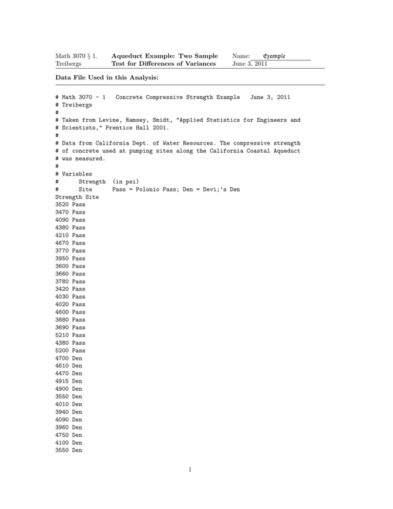
Math 3070 § 1. Treibergs Aqueduct Example: Two Sample Test for Differences of Variances Name: Example June 3, 2011 Data File Used in this Analysis: # Math 3070 - 1 Concrete Compressive Strength Example June 3, 2011 # Treibergs # # Taken from Levine, Ramsey, Smidt, "Applied Statistics for Engineers and # Scientists," Prentice Hall 2001. # # Data from California Dept. of Water Resources. The compressive strength # of concrete used at pumping sites along the California Coastal Aqueduct # was measured. # # Variables # Strength (in psi) # Site Pass = Polonio Pass; Den = Devi;’s Den Strength Site 3520 Pass 3470 Pass 4090 Pass 4380 Pass 4210 Pass 4670 Pass 3770 Pass 3950 Pass 3600 Pass 3660 Pass 3780 Pass 3420 Pass 4030 Pass 4020 Pass 4600 Pass 3880 Pass 3690 Pass 5210 Pass 4380 Pass 5200 Pass 4700 Den 4610 Den 4470 Den 4915 Den 4900 Den 3550 Den 4010 Den 3940 Den 4090 Den 3960 Den 4750 Den 4100 Den 3550 Den 1 3830 3950 3600 4030 5330 5460 3760 Den Den Den Den Den Den Den R Session: R version 2.11.1 (2010-05-31) Copyright (C) 2010 The R Foundation for Statistical Computing ISBN 3-900051-07-0 R is free software and comes with ABSOLUTELY NO WARRANTY. You are welcome to redistribute it under certain conditions. Type ’license()’ or ’licence()’ for distribution details. Natural language support but running in an English locale R is a collaborative project with many contributors. Type ’contributors()’ for more information and ’citation()’ on how to cite R or R packages in publications. Type ’demo()’ for some demos, ’help()’ for on-line help, or ’help.start()’ for an HTML browser interface to help. Type ’q()’ to quit R. [R.app GUI 1.34 (5589) i386-apple-darwin9.8.0] [Workspace restored from /home/1004/ma/treibergs/.RData] > tt <- read.table("M3074AqueductData.txt", header=T) > attach(tt) > tt Strength Site 1 3520 Pass 2 3470 Pass 3 4090 Pass 4 4380 Pass 5 4210 Pass 6 4670 Pass 7 3770 Pass 8 3950 Pass 9 3600 Pass 10 3660 Pass 11 3780 Pass 12 3420 Pass 13 4030 Pass 14 4020 Pass 2 15 16 17 18 19 20 21 22 23 24 25 26 27 28 29 30 31 32 33 34 35 36 37 38 39 40 4600 3880 3690 5210 4380 5200 4700 4610 4470 4915 4900 3550 4010 3940 4090 3960 4750 4100 3550 3830 3950 3600 4030 5330 5460 3760 Pass Pass Pass Pass Pass Pass Den Den Den Den Den Den Den Den Den Den Den Den Den Den Den Den Den Den Den Den > > ####################### GET A SENSE OF THESE DATA #################################### > tapply(Strength,Site,summary) $Den Min. 1st Qu. Median Mean 3rd Qu. Max. 3550 3912 4060 4275 4712 5460 $Pass Min. 1st Qu. 3420 3682 Median 3985 Mean 3rd Qu. 4076 4380 Max. 5210 > # Their variances? > > tapply(Strength,Site,var) Den Pass 334540.7 277676.6 > > title("Boxplot of Compressive Strength at Pumping Sites") 3 4500 3500 4000 Strength 5000 5500 Boxplot of Compressive Strength at Pumping Sites Den Pass Site > # Pick off the measurements at the two sites. > > y1 <- tt[Site=="Pass",1] > y1 [1] 3520 3470 4090 4380 4210 4670 3770 3950 3600 3660 3780 3420 4030 4020 4600 [16] 3880 3690 5210 4380 5200 > y2 <- tt[Site=="Den",1]; y2 [1] 4700 4610 4470 4915 4900 3550 4010 3940 4090 3960 4750 4100 3550 3830 3950 [16] 3600 4030 5330 5460 3760 > qqnorm((y1-mean(y1))/sd(y1),main="Normal QQ: Strength at Polonio Pass", + ylab="Standardized Strength") 4 > > + > > abline(0,1,col=2) qqnorm((y2-mean(y2))/sd(y2),main="Normal QQ: Strength at Devil’s Den", ylab="Standardized Strength") abline(0,1,col=4) # M3074Aqueduct2.pdf > # > Neither data shows nonnormal tendencies. We may assume both samples are normal. 5 > ############################## TEST WHETHER VARIANCES ARE DIFFERENT ########################## > > var.test(y1,y2) F test to compare two variances data: y1 and y2 F = 0.83, num df = 19, denom df = 19, p-value = 0.6888 alternative hypothesis: true ratio of variances is not equal to 1 95 percent confidence interval: 0.3285333 2.0970130 sample estimates: ratio of variances 0.8300233 > # High p-value: we cannot reject null hypothesis that the ratio of variances is one. > ###################### TEST WHETHER VARIANCES ARE DIFFERENT > n1 <- length(y1); n1 [1] 20 > n2 <- length(y2); n2 [1] 20 > > # ratio of variances. > > F <- var(y1)/var(y2); F [1] 0.8300233 BY HAND ########################## > # For two sided test, the lower and upper critical values are > alpha <- .05 > critf1 <- qf(alpha/2,n1-1,n2-1);critf1 [1] 0.3958122 > critf2 <- qf(alpha/2,n1-1,n2-1,lower.tail=F);critf2 [1] 2.526451 > > # Note that since n1=n2, critf2 = 1/ critf21 > 1/critf2 [1] 0.3958122 > # 2-sided CI on F = (s2^2/sigma1^2)/(s2^2/sigma2^2) ~ f(num df=n1-1, denom df = n2-1) > # so with significance alpha, critf1 < F < critf2. Solve ineq for sigma1^2/sigma2^2: > c(F/critf2,F/critf1) [1] 0.3285333 2.0970130 > > # The two sided p-value = P(f below F or above 1/F) > pv <- pf(F,n1-1,n2-1)+ pf(1/F,n1-1,n2-1,lower.tail=F);pv [1] 0.6888292> 6


