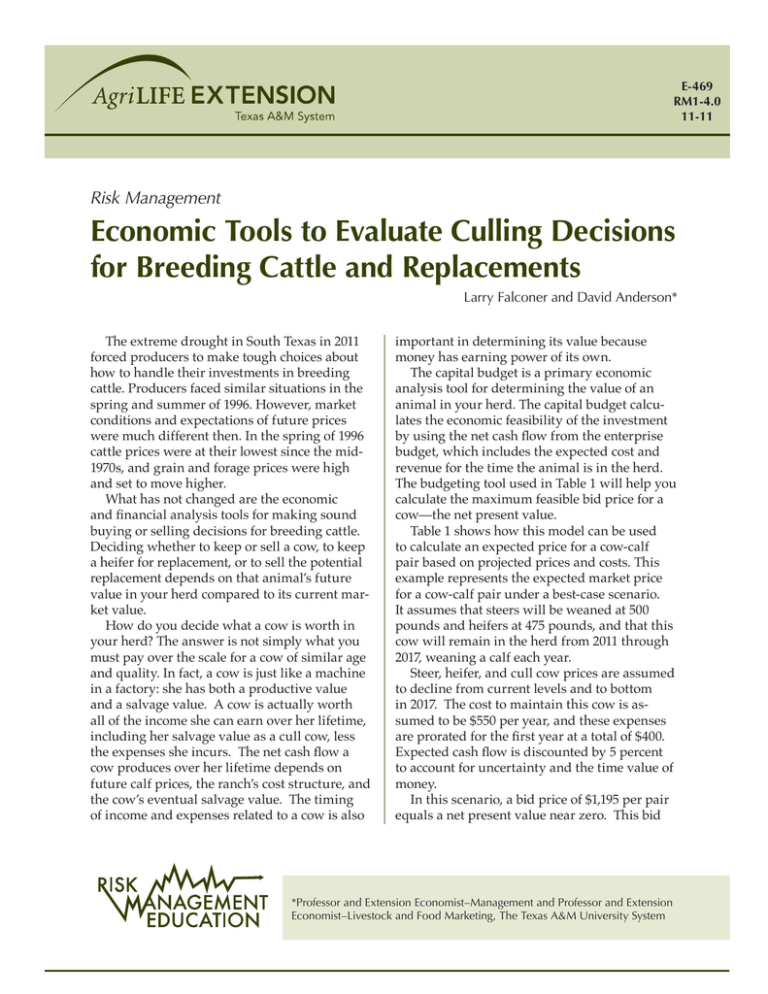
E-469
RM1-4.0
11-11
Risk Management
Economic Tools to Evaluate Culling Decisions
for Breeding Cattle and Replacements
Larry Falconer and David Anderson*
The extreme drought in South Texas in 2011
forced producers to make tough choices about
how to handle their investments in breeding
cattle. Producers faced similar situations in the
spring and summer of 1996. However, market
conditions and expectations of future prices
were much different then. In the spring of 1996
cattle prices were at their lowest since the mid1970s, and grain and forage prices were high
and set to move higher.
What has not changed are the economic
and financial analysis tools for making sound
buying or selling decisions for breeding cattle.
Deciding whether to keep or sell a cow, to keep
a heifer for replacement, or to sell the potential
replacement depends on that animal’s future
value in your herd compared to its current market value.
How do you decide what a cow is worth in
your herd? The answer is not simply what you
must pay over the scale for a cow of similar age
and quality. In fact, a cow is just like a machine
in a factory: she has both a productive value
and a salvage value. A cow is actually worth
all of the income she can earn over her lifetime,
including her salvage value as a cull cow, less
the expenses she incurs. The net cash flow a
cow produces over her lifetime depends on
future calf prices, the ranch’s cost structure, and
the cow’s eventual salvage value. The timing
of income and expenses related to a cow is also
important in determining its value because
money has earning power of its own.
The capital budget is a primary economic
analysis tool for determining the value of an
animal in your herd. The capital budget calculates the economic feasibility of the investment
by using the net cash flow from the enterprise
budget, which includes the expected cost and
revenue for the time the animal is in the herd.
The budgeting tool used in Table 1 will help you
calculate the maximum feasible bid price for a
cow—the net present value.
Table 1 shows how this model can be used
to calculate an expected price for a cow-calf
pair based on projected prices and costs. This
example represents the expected market price
for a cow-calf pair under a best-case scenario.
It assumes that steers will be weaned at 500
pounds and heifers at 475 pounds, and that this
cow will remain in the herd from 2011 through
2017, weaning a calf each year.
Steer, heifer, and cull cow prices are assumed
to decline from current levels and to bottom
in 2017. The cost to maintain this cow is assumed to be $550 per year, and these expenses
are prorated for the first year at a total of $400.
Expected cash flow is discounted by 5 percent
to account for uncertainty and the time value of
money.
In this scenario, a bid price of $1,195 per pair
equals a net present value near zero. This bid
*Professor and Extension Economist–Management and Professor and Extension
Economist–Livestock and Food Marketing, The Texas A&M University System
value leads to an internal rate of return of 5 percent
during the 7 year period. These results indicate
that a bid of $1,195 per pair would be the maximum
feasible bid price in this example. At any price above
$1,195, the producer would be better off selling the
pair. If drought increases the maintenance cost in
the first year, it would be even more advantageous to
sell the cow-calf pair at any price above $1,195.
In early May 2011, young to middle-aged cow-
calf pairs with 100 to 300 pound calves were selling
in South Texas for $900 to almost $1,100 per pair.
The high end of this range is slightly below the
maximum feasible bid price of $1,195. Under normal
circumstances, the producer would be better off
keeping the pair at those sub-$1,100 prices.
However, current drought conditions make it
likely that the prorated operating cost for 2011 is too
low. In our example, there is only $95 per pair in cur-
Table 1. Cow bid price estimate calculator example.
Steer weight
500
Cull cow sale weight (lb/head)
Heifer weight
475
Number of calving opportunities (yr)
$1,195
Discount rate (%)
Pair price
1,000 Lb.
7
Net present
value (NPV)
5.00 %
($0.09)
2011
2012
2013
2014
2015
2016
2017
Year 1
Year 2
Year 3
Year 4
Year 5
Year 6
Year 7
100
100
100
100
100
100
100
Steers price ($/cwt)
$140
$150
$155
$133
$130
$126
$126
Heifer price ($/cwt)
$134
$144
$149
$127
$124
$120
$120
$0
$0
$0
$0
$0
$0
$60
Gross receipts (calf sales)
$668
$717
$741
$634
$620
$600
$600
Cow operating cost/year
$400
$550
$550
$550
$550
$550
$550
Net above operating cost
$268
$167
$191
$84
$70
$50
$50
$0
$268
$167
$191
$84
$70
$50
$50
$0
$0
$0
$0
$0
$0
$0
$600
$0
Year
Calf crop or weaning %
Cull cow price ($/cwt)
$0
Financing information
Net Cash Flow
Cow Salvage Value
Pre-tax cash flows
Year 0
Year 1
Year 2
Year 3
Year 4
Year 5
Year 6
Year 7
($1,195)
$268
$167
$191
$84
$70
$50
$650
*Comments regarding this investment scenario. The analysis of this scenario is on a pre-tax basis.
The negative net present value indicates that the price of $1,195 per head is too high.
This investment has an internal rate of return of 5.0%.
This investment has a payback period of 7 years.
The positive cash flows across the planning horizon indicate that this investment is financially feasible.
2
$0
rent value to cover any additional costs due to the
drought. If $95 would not cover extra expenses, it
would be better to sell the pair now. Also, if the cow
missed weaning a calf in any subsequent year, the
model would generate a sell signal.
This example shows how a cattle producer can use
an economic model to evaluate alternatives when
faced with selling decisions in response to drought.
For tools like the one in Table 1 to yield accurate
data on which to base decisions, producers must use
data that is specific to their operation. Producers
should manipulate production, cost and output price
assumptions to see how those changes would affect
the decision variables.
The expected value of different types of cows in
your herd depends on factors that are uncertain. Because of the uncertainty, many people consider this
type of planning a waste of effort. The future seldom
unfolds exactly as planned, and expecting current
conditions to prevail is unreasonable. The planning
process, however, need not yield an exact prediction
to be valuable.
There is no method that will consistently provide
the best culling strategy. Given the differences in
age composition of herds and the physical resources
for a particular ranch, the “cull half” and “cull to
pay feed” may not be enough for a younger herd
or may be too much for an older herd. However,
the capital budget tool can help you calculate what
might be best for your situation. The “right” answer
depends on the cost structure for your ranch and
what you expect future prices to be.
These tools are available through your local
county Extension office or at http://agecoext.tamu.edu/
resources/software.html
Partial funding support has been provided by the
Texas Corn Producers, Texas Farm Bureau, and
Cotton Inc.–Texas State Support Committee.
Produced by Texas A&M AgriLife Communications
Extension publications can be found on the Web at AgriLifeBookstore.org
Visit the Texas AgriLife Extension Service at AgriLifeExtension.tamu.edu
Educational programs of the Texas AgriLife Extension Service are open to all people without regard to race, color, sex, disability, religion, age, or national origin.
Issued in furtherance of Cooperative Extension Work in Agriculture and Home Economics, Acts of Congress of May 8, 1914, as amended, and June 30, 1914, in
cooperation with the United States Department of Agriculture. Edward G. Smith, Director, Texas AgriLife Extension Service, The Texas A&M System.
Revision