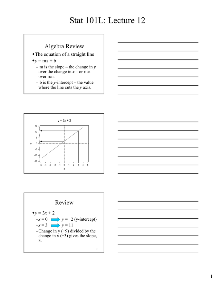
Stat 101L: Lecture 12
Algebra Review
The equation of a straight line
y = mx + b
– m is the slope – the change in y
over the change in x – or rise
over run.
– b is the y-intercept – the value
where the line cuts the y axis.
1
y = 3x + 2
15
10
y
5
0
-5
-10
-15
-5
-4
-3
-2
-1
0
1
2
x
3
4
5
2
Review
y = 3x + 2
–x = 0
y = 2 (y-intercept)
–x = 3
y = 11
– Change in y (+9) divided by the
change in x (+3) gives the slope,
3.
3
1
Stat 101L: Lecture 12
Linear Regression
Example: Tar (mg) and CO
(mg) in cigarettes.
– y, Response: CO (mg).
– x, Explanatory: Tar (mg).
– Cases: 25 brands of cigarettes.
4
Correlation Coefficient
Tar and nicotine
r
z
x
zy
n 1

22 .9796
24
r = 0.9575
5
Linear Regression
There is a strong positive linear
association between tar and
nicotine.
What is the equation of the line
that models the relationship
between tar and nicotine?
6
2
Stat 101L: Lecture 12
Linear Model
The linear model is the
equation of a straight line
through the data.
A point on the straight line
through the data gives a
predicted value of y, denoted ŷ .
7
Residual
The difference between the
observed value of y and the
predicted value of y, ŷ , is
called the residual.
Residual = y  yˆ
8
Residual
9
3
Stat 101L: Lecture 12
Line of “Best Fit”
There are lots of straight lines
that go through the data.
The line of “best fit” is the line
for which the sum of squared
residuals is the smallest – the
least squares line.
10
Line of “Best Fit”
yˆ  b0  b1 x
Least squares
slope:
intercept:
sy
sx
b0  y  b1 x
b1  r
11
Summary of the Data
Tar, x
x  12.216 mg
sx  5.6658 mg
Nicotine, y
y  12.528 mg
s y  4.7397 mg
r  0.9575
12
4
Stat 101L: Lecture 12
Least Squares Estimates
4.7397
 0.801
5.6658
b0  12.528  0.801(12.216)  2.743
b1  0.9575
yˆ  2.743  0.801x
Predicted CO  2.743  0.801* Tar
13
Interpretations
 Slope – for every 1 mg increase in
tar, the CO content increases, on
average, 0.801 mg.
 Intercept – there is not a reasonable
interpretation of the intercept in
this context because one wouldn’t
see a cigarette with 0 mg of tar.
14
Predicted CO = 2.743 + 0.801*Tar
15
5