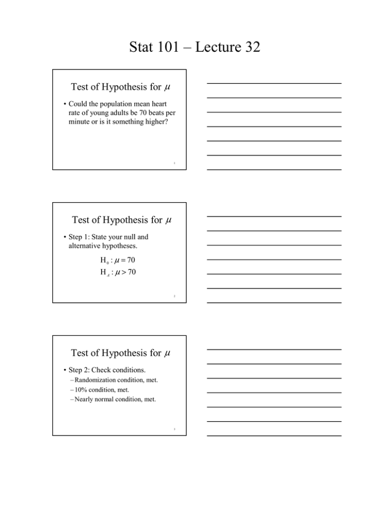
Stat 101 – Lecture 32
Test of Hypothesis for µ
• Could the population mean heart
rate of young adults be 70 beats per
minute or is it something higher?
1
Test of Hypothesis for µ
• Step 1: State your null and
alternative hypotheses.
H 0 : µ = 70
H A : µ > 70
2
Test of Hypothesis for µ
• Step 2: Check conditions.
– Randomization condition, met.
– 10% condition, met.
– Nearly normal condition, met.
3
Stat 101 – Lecture 32
Test of Hypothesis for µ
• Step 3: Calculate the test statistic
and convert to a P-value.
y − µ0
t=
SE( y )
s
SE( y ) =
n
4
Summary of Data
• n = 25
• y = 74.16 beats
• s = 5.375 beats
• SE ( y ) =
s
= 1.075 beats
n
5
Value of Test Statistic
y − µ 0 74.16 − 70
=
SE ( y )
1.075
t = 3.87
t=
Use Table T to find the P-value.
6
Stat 101 – Lecture 32
Table T
One tail probability 0.10
0.05
0.025
0.01
0.005 P-value
df
1
2
3
4
M
24
2.064
2.492
2.797 3.87
The P-value is less than 0.005.
7
Test of Hypothesis for µ
• Step 4: Use the P-value to reach a
decision.
• The P-value is very small,
therefore we should reject the null
hypothesis.
8
Test of Hypothesis for µ
• Step 5: State your conclusion
within the context of the problem.
• The mean heart rate of all young
adults is more than 70 beats per
minute.
9
Stat 101 – Lecture 32
Alternatives
H 0 : µ = µ0
H A : µ < µ0 , P - value = Pr < t
H A : µ > µ0 , P - value = Pr > t
H A : µ ≠ µ0 , P - value = Pr > t
10
JMP:Analyze – Distribution
• Test Mean
t-test
Hypothesized
value
Actual Estimate
df
Std Dev
70 Test
statistic
74.16 Prob > |t|
3.87
0.0007
24 Prob > t
0.0004
5.375 Prob < t
0.9996
11
Another Example
• Is the population mean octane
rating 90 or is it something
different?
12
Stat 101 – Lecture 32
Test of Hypothesis for µ
• Step 1: State your null and
alternative hypotheses.
H 0 : µ = 90
H A : µ ≠ 90
13
Test of Hypothesis for µ
• Step 2: Check conditions.
– Randomization condition, met.
– 10% condition, met.
– Nearly normal condition, met.
14
Normal Quantile Plot
3
.99
2
.95
.90
1
.75
0
.50
.25
-1
.10
.05
-2
.01
-3
6
4
Count
8
2
87
88
89
90
91
92
93
Octane Rating
94
95
15
Stat 101 – Lecture 32
Test of Hypothesis for µ
• Step 3: Calculate the test statistic
and convert to a P-value.
y − µ0
t=
SE( y )
s
SE( y ) =
n
16
Summary of Data
• n = 40
• y = 90.9475
• s = 1.530
• SE ( y ) =
s
= 0.2419
n
17
Value of Test Statistic
y − µ 0 90.9475 − 90
=
SE ( y )
0.2419
t = 3.92
t=
Use Table T to find the P-value.
18
Stat 101 – Lecture 32
Table T
Two tail probability 0.20
0.10
0.05
0.02
0.01
2.021
2.423
2.704
P-value
df
1
2
3
4
M
39
40
3.92
The P-value is less than 0.01.
19
Test of Hypothesis for µ
• Step 4: Use the P-value to reach a
decision.
• The P-value is very small,
therefore we should reject the null
hypothesis.
20
Test of Hypothesis for µ
• Step 5: State your conclusion
within the context of the problem.
• The population mean octane rating
is not 90 but something different.
21
Stat 101 – Lecture 32
Confidence Interval for µ
y − tn*−1SE ( y ) to y + tn*−1SE ( y )
90.9475 ± 2.021(0.2419 )
90.95 − 0.49 to 90.95 + 0.49
90.46 to 91.44
22
Interpretation
• We are 95% confident that the
population mean octane rating is
between
90.46 and 91.44
23
Interpretation
• This confidence interval agrees
with the test of hypothesis.
• 90 is not in the interval and so
must be rejected as a value for the
population mean.
24