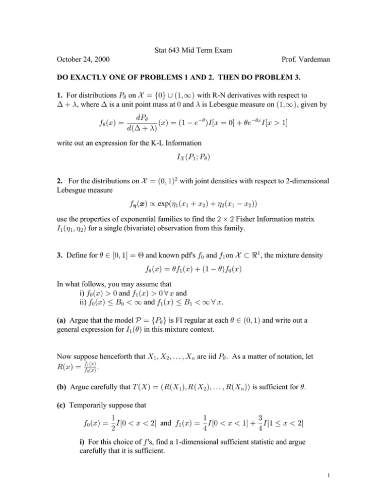
Stat 643 Mid Term Exam
October 24, 2000
Prof. Vardeman
DO EXACTLY ONE OF PROBLEMS 1 AND 2. THEN DO PROBLEM 3.
1. For distributions T) on k œ Ö!× • Ð"ß_Ñ with R-N derivatives with respect to
? € -, where ? is a unit point mass at ! and - is Lebesgue measure on Ð"ß_Ñ , given by
0) ÐBÑ œ
.T)
ÐBÑ œ Ð" • /•) ÑMÒB œ !Ó € )/•)B MÒB ž "Ó
.Ð? € -Ñ
write out an expression for the K-L Information
M\ ÐT" à T) Ñ
2. For the distributions on k œ Ð!ß "Ñ# with joint densities with respect to 2-dimensional
Lebesgue measure
0( ÐBÑ º expa(" ÐB" € B# Ñ € (# ÐB" • B# Ñb
use the properties of exponential families to find the # ‚ # Fisher Information matrix
M" Ð( "ß (#Ñ for a single (bivariate) observation from this family.
3. Define for ) - Ò!ß "Ó œ @ and known pdf's 0! and 0" on k § d" , the mixture density
0) ÐBÑ œ )0" ÐBÑ € Ð" • )Ñ0! ÐBÑ
In what follows, you may assume that
i) 0! ÐBÑ ž ! and 0" ÐBÑ ž ! a B and
ii) 0! ÐBÑ Ÿ F! • _ and 0" ÐBÑ Ÿ F" • _ a B.
(a) Argue that the model c œ ÖT) × is FI regular at each ) - Ð!ß "Ñ and write out a
general expression for M" Ð)Ñ in this mixture context.
Now suppose henceforth that \" ß \# ß á ß \8 are iid T) Þ As a matter of notation, let
VÐBÑ œ 00"! ÐBÑ
ÐBÑ .
(b) Argue carefully that X Ð\Ñ œ ÐVÐ\" ÑßVÐ\# Ñß á ß VÐ\8 ÑÑ is sufficient for ).
(c) Temporarily suppose that
0! ÐBÑ œ
"
"
$
MÒ! • B • #Ó and 0" ÐBÑ œ MÒ! • B • "Ó € MÒ" Ÿ B • #Ó
#
%
%
i) For this choice of 0 's, find a 1-dimensional sufficient statistic and argue
carefully that it is sufficient.
1
ii) Is your statistic from ii) above minimal sufficient? Argue carefully one way or
the other.
It is possible to verify (don't bother to do so here) that provided 0! and 0" both have
second moments, in the obvious notation
E) \" œ )." € Ð" • )Ñ.! and Var) \" œ )5"# € Ð" • )Ñ5## € )Ð" • )ÑÐ." € .# Ñ#
(d) Argue that for problems where ." Á .! , the estimator
)˜ 8 œ
"
.!
\8 •
." • .!
." • .!
(and therefore its truncation to Ò!ß "Ó) is consistent for ) - @.
(e) Suggest a possible improvement over )˜ 8 . Write a recipe for this improvement in as
explicit terms as possible.
(f) Find the form of the likelihood equation in this problem.
Henceforth assume that
"
0! ÐBÑ œ MÒ! • B • "Ó and 0" ÐBÑ œ ŒB € •MÒ! • B • "Ó
#
For this pair of densities, M" Ð)Ñ is as graphed on Figure 1.
(g) Argue carefully that if s)8 is a consistent root of the likelihood equation, it is
asymptotically normal. (You may point to an appropriate theorem, but make it clear that
the hypotheses of that theorem hold.)
(h) A particular sample of size 8 œ "'! in this context has loglikelihood as graphed on
Figure 2. On this plot, the maximum loglikelihood occurs at about ) œ Þ$(*.
P8 ÐÞ$(*Ñ ¸ Þ)" and Pww8 ÐÞ$(*) ¸ • ""Þ&!*Þ Give three different approximate confidence
intervals for ), derived from three different asymptotic approximations.
(i) Consider a Bayes analysis of this problem with a prior distribution uniform on
@ œ Ò!ß "Ó. Figure 3 is a plot of the likelihood for the sample referred to in (h).
i) Give a normal approximation for the posterior probability that ) - ÒÞ%,Þ'Ó based
on a limiting form for the posteriorÞ
ii) Do some appropriate "graphical integration" and find a more or less exact
numerical value for the posterior probability that ) - ÒÞ%,Þ'ÓÞ
2
0.1
0.095
I1( θ ) 0.09
0.085
0.08
0
0.1
0.2
0.3
0.4
0.5
0.6
0.7
0.8
0.9
1
θ
Figure 1
3
1
0.5
0
LogLike( θ ) 0.5
1
1.5
2
0
0.2
0.4
0.6
0.8
1
θ
Figure 2
4
2.5
2.25
2
1.75
1.5
Like( θ ) 1.25
1
0.75
0.5
0.25
0
0
0.1
0.2
0.3
0.4
0.5
0.6
0.7
0.8
0.9
1
θ
Figure 3
5