Stat 643 Spring 2010
Assignment 08
Asymptotic of Likelihood-Based Inference
In the following arguments, we adopt the notations Op (1), op (1). Specifically, we say a sequence of
random variables {Yn } is Op (1), or stochastically bounded, if and only if, ∀ > 0, there exists M > 0
such that P (|Yn | ≤ M ) ≥ 1 − . Note that convergence in distribution implies stochastically bounded.
p
We say {Yn }n≥1 is op (1) if and only if Yn →
− 0. One can see A+L or Shao for references.
65. (a) Let µ be the sum of two measures, one is the Lebesgue measure on (1, ∞), the other is the
point mass measure at 0. Then the R-N derivative of the probability measure of X with
respect to µ is λe−λx I{x 6= 0} + (1 − e−λ )I{x =P0} almost
surely. AdoptPthe notation in
P
n
n
−λ
δ
X
δ
i
i
i
i
(1 − e−λ )n− i δi , where δi =
the class, the likelihood-function is fλ (X ) = P
λ i e
I{Xi 6= 0}. Then under the event M = n − i δi = n, the likelihood function becomes
(1 − e−λ )n , which has no maximizer
∞). In all the other
one of δi
P for λ on (0,P
P cases, at least
n
−λ
is 1, notice that
log fλ (X ) = i δi log(λ) − λ i δi Xi + (n − i δi ) log(1 − e ). Further,
P
P
P
∂ n
n
i δi
0, the score
f (X ) = λ − i δi Xi + (n − i δi )/(1 − e−λ ). As we could see, when λ →P
∂λ λ
function converges to +∞, and when λ → ∞, the score function converges to − i δi Xi . By
the intermediate value theorem, the likelihood equation has at least one root on (0, ∞) in this
case. Therefore, Pλ (MLE exists) ≥ Pλ (M < n) = 1 − Pλ (Xi = 0, ∀i) = 1 − (1 − e−λ )n → 1 as
n → ∞, for any λ > 0.
(b) Let Tn = − log(1 − M/n), then by SLLN, M/n → 1 − e−λ , w.p.1., which implies Tn
converges
to λP almost surely
Pλ . A “1-step Newton improvement” would then be λ̃n =
P
P
Xi +(n− i δi )n/M
i δi /Tn − i δiP
P
Tn − − δi /T 2 −(n− δi )(n/M −1)n/M .
i
n
i
(c) In the event that the MLE exists, we can use the Newton-Raphson method with Tn as the
starting value. Basically, we are repeating the procedure as done in (b) and update each step
with a “1-step newton improvement” adjusted value.
(d) For a (1 − α)100% asymptotic confidence interval, we can use λ̂n ± z1−α/2 {nI1 (λ̂n )}−1/2 and
λ̂nP
±z1−α/2 {−L00n (λ̂nP
)}−1/2 , where Ln is the log-likelihood function. More specifically, L00n (λ) =
− i δi /λ2 − (n − i δi )e−λ /(1 − e−λ )2 , nI1 (λ) = Eλ (−L00n (λ)) = ne−λ /λ2 + ne−λ /(1 − e−λ ).
66. The log-likelihood function for the uncensored data (suppose the dominating measure is the
Lebesgue measure on R+ )is
n
X
`n (λ) = n log λ − λ
Xi
(1)
i=1
1
−30
−50
−70
Loglikelihood
−90
Uncencored
Cencored
0
1
2
3
4
λ
Figure 1: Log-likelihood function for the uncensored and censored data.
For the censored data, the R-N derivative of XI{X > 1}, with respect to the σ-finite measure
that is the sum of Lebesgue measure on (0, ∞) and point mass measure at 0, is (see problem 35)
X
X
X
`∗n (λ) =
δi log λ − λ
δi Xi + (n −
δi ) log(1 − e−λ ),
(2)
i
i
i
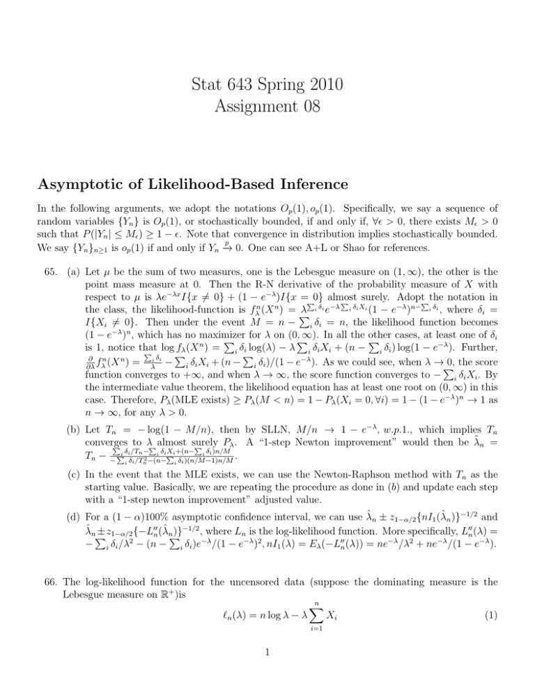
where δi = I{Xi > 1}. For the data given in this problem, their likelihood function is shown in
the Figure 1.
(a) Given the uncensored data, the 90% two-sided confidence set for λ is {λ | χ21,0.05 ≤ 2{`n (λ̂) −
`n (λ)} ≤ χ21,0.95 }. In this case, λ̂ = 1/X̄n = 0.9341, `n (λ̂) = −21.3625, χ21,0.05 = 0.00393, χ21,0.95 =
3.84146. Then one can solve some nonlinear equations and get the confidence interval of λ
(OK, a huge literature that is not the focus of this course!).
(b) Their relationship can be seen in Figure 1.
(c) The Fisher-information in λ about XI{X > 1} evaluated at λ = λ0 is
I1∗ (λ0 ) = Eλ0 δ/λ20 + (1 − δ)eλ0 /(eλ0 − 1)2 = e−λ0 /λ20 + e−λ0 /(1 − e−λ0 ).
2
(3)
q
Two different approximate (Wald) 90% confidence sets would be λ̃ ± z0.05 nI1 (λ̃) and
q
λ̃ ± z0.05 −`00n (λ̃), where λ̃ is the maximum likelihood estimator for censored data.
67. So θ = (p1 , p2 , p3 , p4 )0 and the parameter space Θ is [0, 1]4 . The hypothesis testing problem here
is H0 : θ ∈ Θ0 vs H1 : θ ∈
/ Θ0 , where Θ0 = {(p1 , p2 , p3 , p4 ) ∈ Θ | p1 = p2 , p3 = p4 }.
(a) The likelihood function is
fθn (X n )
=
4 Y
n
Xi
i=1
i
pX
i (1
− pi )
n−Xi
.
(4)
Then the LRT corresponding to this hypothesis testing problem is
4
Y
supθ∈Θ fθn (X n )
=
LRT =
supθ∈Θ0 fθn (X n ) i=1
2Xi
X[i/3]+1 + X[i/3]+2
Xi 2n − 2Xi
2n − X[i/3]+1 − X[i/3]+2
n−Xi
, (5)
where [i/3] stands for the integer part of i/3, e.g. [1/3] = [2/3] = 0, [3/3] = [4/3] = 1.
The log-likelihood ratio would then be the sum of the following two terms
2
X
i=1
4
X
Xi log{2Xi /(X1 + X2 )} + (n − Xi ) log{(2n − 2Xi )/(2n − X1 − X2 )}
(6)
Xj log{2Xj /(X3 + X4 )} + (n − Xj ) log{(2n − 2Xj )/(2n − X3 − X4 )}.
(7)
j=3
They corresponds to the logs of independent LRT statistics for H0 : p = p2 and H0 : p3 = p4
respectively.
1 −1 0 0
(b) h(θ) = (p1 − p2 , p3 − p4 ) and H(θ) =
, and FI is I(θ) = diag(n/{p1 (1 −
0 0 1 −1
p1 )}, n/{p2 (1 − p2 )}, n/{p3 (1 − p3 )}, n/{p4 (1 − p4 )}) Then the Wald statistic is
!
n2
X1 −X2
0
X1 (n−X1 )+X2 (n−X2 )
X3 −X4
X1 −X2
n
(8)
Wn =
X3 −X4
n2
n
n
.
0
n
X (n−X )+X (n−X )
3
3
3
3
A simplification gives us
√
√
{ n(X1 − X2 )/n}2
{ n(X3 − X4 )/n}2
Wn =
+
.
X1 (n − X1 )/n + X2 (n − X2 )/n X3 (n − X3 )/n + X4 (n − X4 )/n
(9)
d
Then we can see that, under H0 , Wn →
− χ22 .
(c) Under H0 , θ̃ = (p̃1 , p̃2 , p̃3 , p̃4 )0 , where p̃1 = p̃2 = (X1 + X2 )/(2n), p̃3 = p̃4 = (X3 + X4 )/(2n).
Then the score test statistic is
Vn =
(X1 − np̃1 )2 (X2 − np̃2 )2 (X3 − np̃3 )2 (X4 − np̃4 )2
+
+
+
.
np̃1 (1 − p̃1 )
np̃2 (1 − p̃2 )
np̃3 (1 − p̃3 )
np̃4 (1 − p̃4 )
3
(10)
After some algebra, it becomes
Vn =
(X3 − X4 )2
(X1 − X2 )2
+
,
2np̃1 (1 − p̃1 ) 2np̃3 (1 − p̃3 )
(11)
which converges to χ22 under H0 .
68. (a) 1/Pθ ({0}) = 1 + eθ + e2θ , thus a moment estimator of θ based on n0 is
(
)
p
−1 + 4n/n0 − 3
θ̂ = log
.
(12)
2
p
√
Denote g(t) = log{(−1 + 4/t − 3)/2}. As n(n0 /n − Pθ ({0})) is asymptotically normal,
√
and g 0 (Pθ ({0})) 6= 0. By delta method, n(θ̂ − θ) = Op (1), specifically, it is asymptotically
normally distributed.
P
P
P
(b) Note that i I{Xi = 1}θ + 2 i I{Xi = 2} = i Xi . The log-likelihood is
X
Ln (θ) = θ
Xi − n log(1 + eθ + e2θ )
(13)
i
L0n (θ) =
X
i
Xi −
neθ + 2ne2θ
1 + eθ + e2θ
(14)
(neθ + 4ne2θ )(1 + eθ + e2θ ) − n(eθ + 2e2θ )2
(1 + eθ + e2θ )2
(15)
∗
L0n (θ̂n ) = L0n (θ) + (θ̂n − θ)L00n (θ) + (θ̂n − θ)2 L000
n (θn )/2,
(16)
L00n (θ) =
If we write
where θn∗ is some estimator between θ̂n and θ0 . Then we have
(
) √
√ 0
∗
√
nLn (θ) √
L00n (θ)
n(θ̂n − θ)2 L000
n (θn )
n(θ̃n − θ) =
+ n(θ̂n − θ) 1 −
−
.
−L00n (θ̂n )
L00n (θ̂n )
2L00n (θ̂n )
(17)
It can be seen that the last two terms of the above expression is op (1) under the conditions
√
p
d
given. Moreover, it can be verified that n{L0n (θ)/n} →
− N (0, I1 (θ)) and −L00n (θ̂n )/n →
− I1 (θ),
thus the result follows.
(c) The likelihood equation is
(2 − x̄)e2θ + (1 − x̄)eθ − x̄ = 0.
When x̄ ∈ (0, 2), the solution is
(
)
p
x̄ − 1 + (1 − x̄)2 + 4x̄(2 − x̄)
b
θ̂ = log
.
2 − x̄
(18)
(19)
√ b
d
− N (0, 1/I1 (θ)) in θ probability. It suffices to verify the condiTo show that n(θ̂n − θ) →
tions of Theorem 173 (which would be easier than proving directly). Conditions 1-5 can be
b
easily verified to be true. Then Pθ (θ̂n is a root of likelihood equation) ≥ Pθ (0 < X̄ < 2) →
1, as n → ∞. Moreover, as x̄ converges to (eθ + 2e2θ )/(1 + eθ + e2θ ) almost surely. Plug the
b
limit back into the above equation, we get θ̂ converges to θ almost surely.
4
(d) The FI is I1 (θ) = V arθ (X) = eθ (1 + 4eθ + e2θ )/(1 + eθ + e2θ )2 . Then any consistent estimator
p
p
of θ say θ̃n such that θn →
− θ, I1 (θ̃n ) →
− I1 (θ). And the observed fisher information is
−L00n (θ)/n = eθ (1+4eθ +e2θ )/(1+eθ +e2θ )2 , which is exactly I1 (θ). Thus their approximations
b
are the same. If we use θ̂n , then
√
(x̄ − 1) + −3x̄2 + 6x̄ + 1
b
√
I1 (θ̂n ) = x̄ 1 − x̄ + 2
.
(20)
x̄ + 2 −3x̄2 + 6x̄ + 1
69. Without loss of generality, assume that h(x) = 1 (otherwise consider µ̃(A) =
this one-parameter density, the R-N derivative has the form
R
A
hdµ). Then for
fη (x) = K(η) exp{ηT (x)}, a.e.(µ),
(21)
R
where K(η) is the normalizing constant. The parameter space is Γ = η | exp{ηT (x)}dµ(x) < ∞ .
(a) For any η0 in the interior of Γ, consider the open neighborhood of η0 , O = (η0 − , η0 + ).
First of all, fη (x) > 0 ∀x ∈ X and η ∈ O. Second, by DCT, fη Rhas first partial derivative
at
R η0 , especially, when taking derivative on both sides of 1 = fθ (x)dµ(x), we get 0 =
∂fη (x)/∂η|η=η0 dµ(x). Thus P is FI regular
at every η0 in the interior of Γ. (The detail for
R
applying DCT is like Rthis. Let g(η) = exp{ηT (x)}dµ(x), then for η ∈ O, g(η) < ∞. Also
{g(η+h)−g(η)}/h = exp{ηT (x)}·{(exp(ηh)−1)/h}dµ(x). Then notice that (exp(ηh)−1)/h
is actually bounded for small enough h and all η ∈ O).
(b) Because of (a), by definition of Fisher Information, the fisher information in X about η
evaluated at η0 is
2
Z ∂{log{K(η)} + ηT (x)} K(η0 ) exp{η0 T (x)}dµ(x).
(22)
I(η0 ) =
∂η
η=η0
R
As 0 = ∂fη (x)/∂η|η=η0 dµ(x), some algebra work will give us K 0 (η0 )/K(η0 ) = −Eη0 {T (X)}.
Thus the above expression simplifies to I(η0 ) = V arη0 {T (X)}.
(c)
Z
I(η0 , η) =
fη (x)
dµ(x) =
fη0 (x) log 0
fη (x)
Z K(η0 )
log
+ (η0 − η)T (x) fη0 (x)dµ(x),
K(η)
(23)
which is log{K(η0 )/K(η)} + (η0 − η)Eη0 {T (X)}.
(d) The likelihood equation is
nK 0 (η)/K(η) +
X
T (Xi ) = 0
(24)
i
(e) Eη0 | log fη (X)| ≤ | log K(η)| + |η0 |Eη0 |T (X)|. Therefore, all conditions of Theorem 170 are
met.
(f) The general form of “one-step Newton improvement” would be
P
K 0 (η̃)
+ n1 i T (Xi )
K(η̃)
η̃ − n
o2
00 (η̃)
K 0 (η̃)
− KK(η̃)
K(η̃)
5
(25)
(g) The proof is straightforward by applying DCT with similar approach as in part (a).
70. To rigorously argue this, define the following set
An = {θ̂n is a root of likelihood equation} ∩ {Ln (θ) is unimodal},
(26)
then limn→∞ Pθ0 (An ) = 1. Then for any random variable Tn , we can claim that |Tn IAn − Tn | =
op (1), in θ0 probability. This is because, for any > 0,
Pθ0 {|Tn IAn − Tn | > } ≤ Pθ0 {Acn } → 0, as n → ∞.
(27)
Therefore, we only need to consider 2IAn {Ln (θ̂n ) − maxθ<θ0 Ln (θ)} here, which equals to 2I{θ0 <
√
d
θ̂n }{Ln (θ̂n ) − Ln (θ0 )}. Also, Theorem 173 says n(θ̂n − θ0 ) →
− N (0, I1−1 (θ0 )) in θ0 probability.
Further, under conditions of Theorem 173, Taylor expansion says Ln (θ0 ) − Ln (θ̂n ) = L0n (θ̂n )(θ0 −
θ̂n ) + 21 L00n (θn∗ )(θ̂n − θ0 )2 , where θn∗ is between θ̂n and θ0 . Therefore, in θ0 probability, 2I{θ0 <
p
p
00 ∗ )/n
d
n
θ̂n }{Ln (θ̂n ) − Ln (θ0 )} = −LIn1(θ
− I{Z > 0}Z 2 ,
I{ nI1 (θ0 )(θ̂n − θ0 ) > 0}{ nI1 (θ0 )(θ̂n − θ0 )}2 →
(θ0 )
where Z ∼ N (0, 1).
p
71. By slustky’s theorem, itP
suffices to prove that, in θ0 , −n−1 L00n (θ̂n ) →
− I1 (θ0 ). Note that n−1 |L00n (θ̂n )−
00
−1
00
−1 00
−1
00
Ln (θ0 )| ≤ |θ̂n − θ0 |n
i M (Xi ) = op (1). Therefore, −n Ln (θ̂n ) = −n {Ln (θ̂n ) − Ln (θ0 )} −
p
n−1 L00n (θ0 ) = op (1) − n−1 L00n (θ0 ) →
− I1 (θ0 ).
72. The hypothesis 1-5 of Theorem 173 guarantee that L0n (Tn ) = L0n (θ0 ) + L00n (θn∗ )(Tn − θ0 ), where θn∗
is between Tn and θ0 . Plug this into the one-step newton improvement formula, we have
√ 0
√
√
L00n (θn∗ )
nLn (θ0 )
n(θ̄n − θ0 ) = n(Tn − θ0 ) 1 − 00
.
(28)
−
Ln (Tn )
L00n (Tn )
√
Notice that Tn = θ0 + Op (n−1/2 ) (a more general condition than n(Tn − θ0 ) converges in disin problem 72,
tribution). Then θn∗ = θ0 + Op (n−1/2 ). One can use the same argument as √
00
00
00
00 ∗
(θ
)
+
o
(1),
which
means
)
=
L
(θ
and
see
that
L
(T
)
=
L
(θ
)
+
o
(1),
L
n(θ̄n − θ0 ) =
p
p
n n
n 0
n 0
n n
√
00 ∗
00
n(Tn − θ0 ) {1 − Ln (θn )/Ln (Tn )} = op (1). The result then follows, by slutsky’s theorem, from the
√
p
d
− I1 (θ0 ), n{n−1 L0n (θ0 ) − 0} →
facts that −n−1 L00n (Tn ) →
− N (0, I1 (θ0 )), in θ0 probability.
6